
2.6 Georeference Raster Maps
Before GIS, there was cartography. For centuries, geographic information has been stored in maps. In the 20th Century, aerial photography added realistic views of the landscape in chemically developed analog imagery. Printed maps and photos can be important sources of data, especially regarding historic features, but also contemporary ones for which data files may not be available.
In order to extract data from a printed map or aerial photograph, it must first be scanned to turn it into a raster image. The raster image can then be georeferenced in GIS software to add spatial information that allows it to be shown in the correct location. This section covers the georeferencing process. The final data extraction step is digitizing, which will be covered in the next section.
Section Outcomes
In this section, you will:
- Add an unreferenced image to ArcGIS Pro
- Roughly align the image to a reference basemap
- Add reference data
- Add control points
- Evaluate control points
- Save a georeferenced copy of the image
 Add an unreferenced image to ArcGIS Pro
You can georeference any map or vertically-oriented aerial image. You can look online for a map or image you would like to use, or scan a paper map (or a piece of one) using a flatbed scanner hooked up to a computer. Do not use a photograph of a map unless you have access to special photography equipment that holds the camera perfectly still and vertical and the map can be laid perfectly flat underneath, with no bends or folds. Any common image format (JPEG, PNG, GIF, or TIFF) will work for the unreferenced image file. The examples in this section use a map of the U.S.-Canada border from the International Boundary Commission.
1. Acquire an unreferenced map or aerial photo image, and place it in the project folder of the ArcGIS Pro project you will work in.
2. In ArcGIS Pro, add the image to the map.
3. In the Contents pane, right-click the image layer, and click “Zoom To Layer”.
4. Zoom the map out until you can see where the image is in relation to other geographic features.
![]() Teachback 18 — Perception and Interpretation
Teachback 18 — Perception and Interpretation
Roughly align the image to a reference basemap
To set up for georeferencing, you need open ArcGIS Pro’s georeferencing tools and set the map projection. You can then use the positioning tools in the Georeference ribbon tab to roughly align the image to the basemap before fine-tuning its position with control points.
5. In the Imagery ribbon tab, click the Georeference button to open the Georeference tab.
6. If you can, determine what map projection is used by the unreferenced image (read any printed text on the map or any metadata that came with it). If you cannot determine the image’s projection, decide on a projection to use while georeferencing that minimizes distortion in the geographic area covered by the image (zoom to this area of the map if necessary).
7. Set the map’s coordinate system to the projection used by the unreferenced image, or to the projection that you determined best minimizes distortion in the area covered by the image. You can do this following the steps in Section 1.6, or using the Set SRS button in the Georeference ribbon tab.
8. Zoom the map to the area covered by the unreferenced image, if you have not already done so.
9. In the Georeference ribbon tab, click the Fit to Display button.
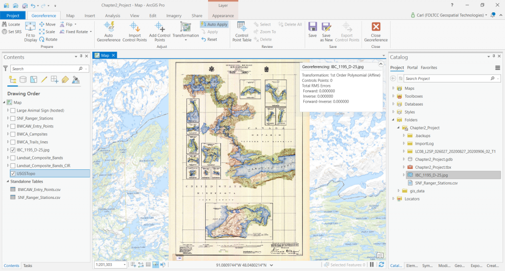
10. If desired, on the Map ribbon tab, change the basemap to one that shows the same features as the unreferenced map or imagery in a comparable way.
11. In the Georeference ribbon tab, use the Move, Scale, and Rotate buttons to adjust the position of the unreferenced image and match it to the correct location as closely as possible. Zoom the map in and out using a mouse wheel or two-finger motion on a trackpad if necessary.
12. When satisfied with the position of the image, click the Explore button in the map ribbon tab to exit the positioning tools.
Add reference data
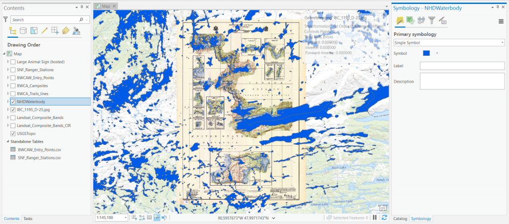
The Georeference tab’s positioning tools allow you to roughly match the image to its location, but an accurate georeferencing job usually requires fine-tuning by comparing the unreferenced image closely to reference data. While a tiled basemap may be adequate for visual reference, vector datasets of features that are shown in the unreferenced image can serve as helpful additional reference data. Roads and water features are commonly used as reference datasets, as they are highly visible and long-lasting landscape features (though beware that they can move over time due to erosion, construction, and natural events).
Only use reference datasets that you trust to be highly accurate, as your georeferencing will only be as accurate as the reference data you use. If needed, you should be able to find and download good reference data from the repositories listed in Appendix A.
![]() Teachback 19 — Intention
Teachback 19 — Intention
- What types of geographic features are visible on your unreferenced image and may be available as vector datasets covering the location of your image?
- Which sources listed in Appendix A could you acquire this reference data from?
13. Acquire at least one vector feature dataset and add it to your ArcGIS Pro project map.
14. Symbolize the new reference layer as desired to make it easily visible against the unreferenced image and basemap (Figure 2.44).
Add control points
With reference data on the map, you can start fine-tuning the georeferencing by adding control points. Control points are points that link locations on the unreferenced image to known locations on the map. They are used to develop a geometric transformation to fit the unreferenced image to the map’s coordinate reference system. The transformation ties each pixel coordinate in the image to a geographic coordinate in the coordinate reference system used by the map.
There are different types of transformations with different levels of complexity in how they distort the original image to fit the coordinate reference system. More complex transformations require more control points. The table below shows the georeferencing transformations available in ArcGIS Pro.
| Transformation (nickname) | Equation form | Minimum control points | Description and use |
|---|---|---|---|
| Zero-order polynomial (shift) | x’ = x + A y’ = y + A |
1 | Shifts image. Used to place already-georeferenced data in its correct location. |
| First-order polynomial (affine) | x’ = Ax + B y’ = Ay + B |
3 | Rotates, shifts, and scales image. Used to fit a geodetically accurate map or orthorectified image to a coordinate reference system that uses its projection. |
| Second-order polynomial (rubber-sheeting) | x’ = Ax2 + Bx + C y’ = Ay2 + By + C |
6 | Rotates, shifts, scales, and warps image. Used to fit a map or orthorectified image to a coordinate reference system that does not match its projection. |
| Third-order polynomial (complex rubber-sheeting) | x’ = Ax3 + Bx2 + Cx + D y’ = Ay3 + By2 + Cy + D |
10 | Warps image in complex ways. Used to fit a non-orthorectified image or spatially inaccurate map to a coordinate reference system. |
| Adjust | Global polynomial + local TIN interpolation | 3 | Performs polynomial transformation, then adjusts areas around each control point using TIN interpolation. Used to fit a non-orthorectified image or spatially inaccurate map to a coordinate reference system. |
| Spline | Piecewise polynomial | 10 | Generates piecewise polynomial equations to exactly fit each control point and interpolate fit between control points. Many control points are needed to get an accurate result. Used to fit a non-orthorectified image or spatially inaccurate map to a coordinate reference system. |
| Projective | Homography | 4 | Preserves straight lines. Used to fit oblique imagery and scanned maps with wrinkles. |
Which transformation you choose depends on how much adjustment is needed to fit the image to the coordinate reference system, and which one appears to do the best job once you have placed several control points.
Where you put these points also matters. Choose specific, permanent ground features that are visible in both the unreferenced image and in the reference data or basemap. If the unreferenced image includes a graticule or coordinate markings, you can place control points at the graticule line intersections or markings and manually enter their coordinates. Control points should be distributed fairly evenly around the image, near the sides as well as in the center. The minimum numbers of control points in the table above will not produce a good result. A good rule of thumb is to place at least 8 control points for simple georeferencing jobs, and 10-16 for more complicated images, such as aerial photos that are not orthorectified. A spline transformation may require 30 or more control points to produce a decent result.
15. In the Appearance ribbon tab for your reference data layer(s), reduce the layer’s transparency so you can see the unreferenced image under its features (and make sure it is above the image in the Contents pane).
16. In the Georeference ribbon tab’s Adjust group, click the Add Control Points button.
17. Zoom the map in until you can see as much detail as possible in the unreferenced image, but the image does not look pixelated.
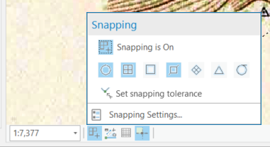
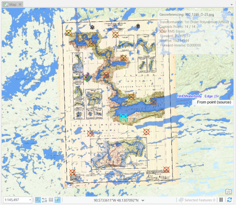
18. In the lower-left corner of the map frame, just to the right of the scale dropdown, click the Snapping button to turn snapping on (if it is not already on). It is also a good idea to turn edge snapping on and vertex snapping off in the snapping options box (Figure 2.45).
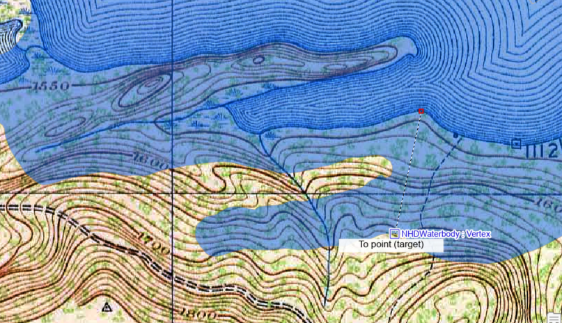
19. Choose a location near one corner of the unreferenced image that you can also see in the reference data, and click on it to place a control point.
20. Find the same location on your reference features and click on it to place the control point’s link (Figure 2.46).
21. In the Contents pane, select the layer of your unreferenced image, then hit the spacebar on your keyboard to turn the layer off and on. You can use this as a shortcut, or check the layer on and off with your mouse, to reveal the underlying basemap while you are georeferencing.
22. Zoom to the opposite corner of the unreferenced image and find a different location to add a control point to. Add its link to the map using either your reference layer or the basemap for reference.
23. If your unreferenced image contains a graticule (coordinate grid) or coordinate marks, locate and zoom to a grid intersection or coordinate mark that you can see the coordinates of using labels along the sides of the image.
24. Place a control point on the grid intersection or coordinate mark, then right-click the map to bring up the “Target Coordinates” window (Figure 2.47).
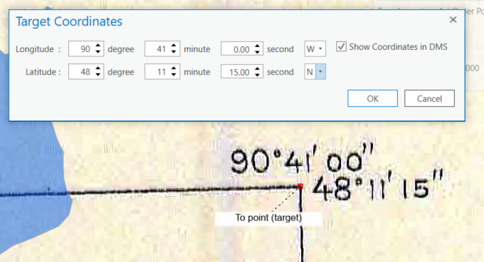
25. If necessary, check the “Show Coordinates in DMS” box, then enter the coordinates shown on the unreferenced image for that location and click “OK”.
26. Continue placing additional control points until you have at least 8 scattered relatively evenly around the image, in corners and along sides as well as in the center (Figure 2.48).
Evaluate Control Points
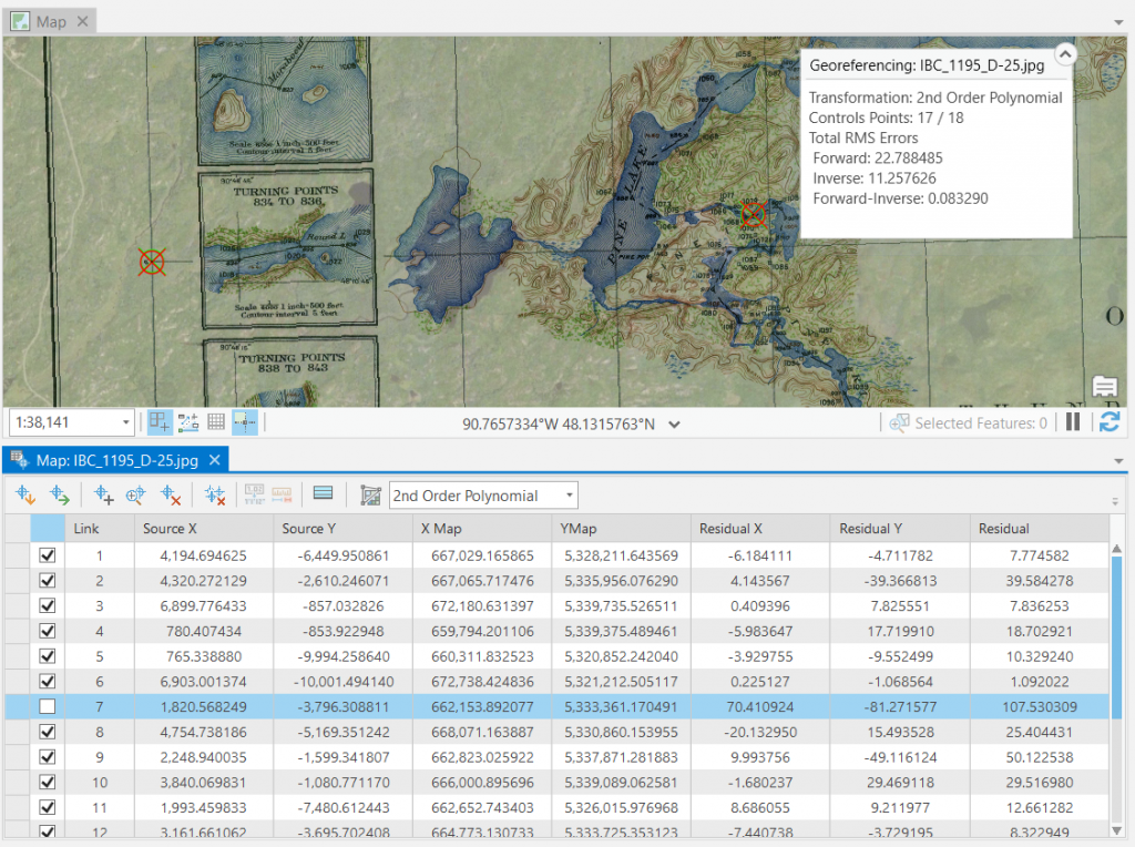
With your control points in place, the next step is to choose the transformation that results in the best fit between the image and the reference data and basemap. To make the georeferencing as accurate as possible, it is also important to evaluate the overall error in the transformation. The error for each control point, or residual, is the distance (in coordinate reference system units) between the control point that was placed on the image and its linked point on the reference map once a transformation is applied. Errors for all control points are totaled as a root mean square error or RMSE, which summarizes the overall error in the transformation.
In ArcGIS Pro, the Georeferencing window in the upper-right corner of the map shows three measures of RMSE: forward, inverse, and forward-inverse. Forward RMSE is measured in coordinate reference system units, while inverse RMSE is measured in image pixels based on the unreferenced image. All three types of RMSE work the same way: the lower the error value, the better the transformation’s fit to the control points.
Individual control points with large residuals may indicate that those control points were not placed properly, and should be deleted and replaced with other nearby control points. This should reduce the RMSE values. Relatively consistent residuals across all control points should result in fairly low RMSE. However, RMSE is never zero except in a spline transformation (because spline perfectly fits all control points, but at the cost of greater error elsewhere). Trying to reduce the RMSE is only helpful to a point, and can actually make the georeferencing less accurate if it causes you to eliminate control points from a difficult area of the image. The most important error evaluation is your judgement of how well the image visually aligns to the reference data and basemap. Once you can no longer get the image to line up any better with the map, it is time to stop making adjustments and export the georeferenced image.
27. In the Map ribbon tab, click the Explore button to stop placing control points and re-enable panning the map.
28. In the Appearance ribbon tab for the image, lower the image transparency, and/or use the Swipe tool to allow you to closely compare different parts of the image to the basemap. You may also wish to experiment with using different basemaps for the comparison.
29. In the Georeference ribbon tab, click the Control Point Table button to open the control point table.
30. Change the Transformation dropdown at the top of the table to a different transformation, then zoom and pan the map to examine how closely different parts of the image fit the reference data and basemap.
31. Determine which transformation best fits the image to the basemap and reference data. Zoom in on different parts of the map to examine the image’s fit in different areas.
29. Examine the residuals of each control point in the right-most column of the table. Look for any very large outliers. If you see any, uncheck the control point on the left side of the table to remove it from the map. Examine how removing it changes the position of the image on the map and the RMS errors shown in the Georeferencing window in the upper-right corner of the map (Figure 2.49).
![]() Teachback 20 — Perception, Interpretation, and Evaluation
Teachback 20 — Perception, Interpretation, and Evaluation
- What transformation results in the best fit of the image to the reference data and basemap?
- What is the forward RMSE of all of your control points in that transformation?
- What is highest residual of any control point? Does it seem to be an outlier—that is, very much greater than any other residuals?
- What happens to the forward RMSE when you uncheck that control point?
- Does unchecking the control point make the image fit better or worse?
- Are there other control points with high residuals that appear to be outliers? If so, what happens when you uncheck them?,
- Do you think any of your control points were placed at the incorrect location (mismatched locations on the image and map)?
- Besides changing the transformation and removing control points, what else could you do to improve the image fit?
30. If you determine that any control points were placed incorrectly, select the offending control point and click the Delete Selected button at the top of the table (which looks like a blue crosshairs with a red X beneath it).
31. If you find areas of the image that do not fit well with the reference data and basemap, and this does not appear to be because of inaccurate control points, place more control points in the poorly-fitting areas to improve their accuracy.
32. When you feel you can no longer improve the fit of the image by adding or removing control points, answer Teachback 21 and move ahead to the next steps.
![]() Teachback 21 — Evaluation
Teachback 21 — Evaluation
- How many control points did you remove and how many did you add before declaring the georeferencing complete?
- Are there parts of the image that still do not quite fit the reference data and basemap? If so, why do you think this is?
Save a georeferenced copy of the image
To make the georeferencing transformation final, the georeferencing (or spatial reference) information must be written to the existing image file, or the image must be exported to a new file along with that information. Because the transformation changes the shape of the image, and pixels remain squares, the image must be resampled. Resampling involves transferring the value of each original pixel to overlying pixels in a new pixel grid.
Simply saving the ArcGIS Pro project will not save the georeferencing of the image. ArcGIS Pro gives you two options for saving your georeferencing work in the Georeference ribbon tab: Save and Save as New. “Save” resamples the image and writes the output along with spatial reference information to the existing image file, overwriting the data that it previously contained. The most common image file formats, including JPEG (.jpg; used mainly for digital photos) and PNG (.png; used primarily for internet graphics), cannot store spatial reference information. Thus, the “Save” option will not work for preserving the georeferencing of these images.
“Save as New” exports the resampled image and spatial reference information to a new raster file. There are many raster file formats that can be used to store spatial reference information. The most common software-agnostic formats for storing georeferenced images are TIFF (.tif or .tiff) and JPEG2000 (.jp2). Both can minimize file sizes without sacrificing any quality using lossless compression algorithms: LZW compression for TIFF files, and wavelet compression for JPEG2000. Other raster formats were created by different software vendors, including Esri’s own native raster formats, and most work fine for storing georeferenced images.
If you would like to save your work but are not yet ready to finalize the image, you can also export the control points as a simple text-based table. They can then be imported to the control points table during your next work session.
33. At the top of the control point table, click the Export Control Points button (the second button from left, which looks like a crosshairs with a green arrow beneath it).
34. In the prompt, choose whether to export only the enabled control points or all control points.
35. Save the control points TXT file to your project folder.
36. In the Georeference ribbon tab, click the Save as New button.
37. In the Export Raster pane, set the “Output Raster Dataset” location to your project folder and enter a filename with a .tif extension. You can edit the file path directly or use the Browse button to do this.
38. Leave the other options in the Export Raster pane set to the defaults, except the Compression Type. Check that “Output Format” is set to “TIFF” and change “Compression Type” to “LZW”. These are the most common format options for geospatial raster images.
39. At the bottom of the Export Raster pane, click “Export”.
40. In the Georeference ribbon tab, click the Close Georeference button.
41. When prompted about unsaved edits, click “Yes” to continue.
42. Remote the original unreferenced image from the Contents pane and save the project.
Further Resources
Data that has been assigned position and coordinate system information so it can be placed at the correct location by GIS software
The process of creating vector feature data by tracing over raster imagery or maps
Accurate geographic data that can be used to georeference an image
Points used to link locations on an unreferenced image to locations in the map's coordinate system
A mathematical equation used to fit a map or image to a particular coordinate reference system
A system for locating features on the Earth, consisting of a datum, projection (if a projected coordinate system), and coordinate grid
A grid of lines on a map showing latitude and longitude coordinates
Imagery that has been processed to remove vertical displacement distortions and align all objects with their correct geographic locations
The location error of a georeferencing control point, or distance between its location on an image to be referenced and its location on the reference map once a transformation is applied
The overall error of a georeferencing transformation, calculated as the square root of the mean square of all control point residuals
