2.5 Use Remotely Sensed Imagery

Thus far, you have primarily worked with vector data. The first four sections of this chapter presented four different ways to create new vector features and layers. However, these are not the only kinds of data that are used in GIS. Instead of discrete features, the raster data model represents the world as continuous surfaces. A raster dataset is a grid of cells or pixels, each of which holds a single attribute value for the geographic area it covers. Because they are continuous, raster datasets are very good at representing continuous phenomena such as terrain, land cover, and atmospheric conditions. For more information on the raster data model, see Section 4.1 of the Campbell and Shin textbook.

The primary source of most raster data is remote sensing. Satellites, airplanes, and drones are used to capture imagery of Earth’s surface and atmosphere. After an initial round of processing, that imagery can be loaded into a GIS project and used for analysis and map-making.

Imagery varies by spatial resolution, or the ground distance covered by each pixel. The larger the ground distance per pixel, the lower the resolution, and the fuzzier the image. Projects covering small areas at large map scales need higher-resolution imagery than those covering large areas at small scales. The quality of imagery can also be affected by atmospheric conditions—if there are clouds or haze between the ground and the sensor, the ground will be obscured in the image.

One free source of imagery is tiled imagery basemaps provided by companies like Esri, Google, Microsoft, and Mapbox. Imagery basemaps generally cover the entire world at resolutions as high as one meter or less, with imagery that has been selected and processed to remove clouds and other flaws. Esri’s imagery basemap is one of the default basemaps provided in ArcGIS Pro; other imagery services can be added to ArcGIS Pro as additional layers.

Imagery basemaps can be extremely useful, but they have downsides. For one thing, the clarity of the imagery can vary from place to place, as can the season the imagery was taken (most places outside of the tropics look very different in summer versus winter). The imagery does not come with any date information, so it can be hard to tell how current it is. Older imagery may be missing features you want to map, like recent forest fire scars or new buildings. You also cannot adjust the appearance of the imagery in any way. If you need more control over the imagery for a project, the best thing to do is download—or even collect—your own.

Quite a lot of low-to-moderate-resolution satellite imagery covering the entire world is freely available online thanks to the U.S. Government’s policy of publishing its data at no cost. It also publishes high-resolution aerial imagery of most areas in the continental U.S. through the USDA National Aerial Imagery Program (NAIP). In other countries, the availability and cost of aerial imagery varies. High-resolution satellite imagery is available for most of the world from private vendors and some governments for a fee. Specific projects that need good-quality, high-resolution imagery from within a certain time frame may require special plane or drone flights.

Remotely sensed imagery is further discussed in Section 4.3 of the Campbell and Shin textbook.

Download Landsat satellite imagery

The Landsat program is a continuous series of scientific remote sensing satellites operated jointly by the United States Geological Survey (USGS) and National Aeronautics and Space Administration (NASA). Landsat 1 was launched into orbit in 1972. It and subsequent Landsat missions have provided imagery of the entire globe at 30-to-120-meter resolution every 16 days since then. As of this writing, two Landsat satellites—Landsats 7 and 8—are in operation, with Landsat 7 scheduled to be retired and Landsat 9 scheduled to launch in late 2021.

Historic and recent Landsat imagery data is available to the public at no charge through the USGS EarthExplorer web portal. You will first need to create a user account for the website. Then you will choose what geographic area to search within, and select imagery to download based on its date and appearance.

Action Sequence

1. In a web browser, visit the USGS EarthExplorer web portal.

2. In the upper-right corner of the page, click “Login”.

3. If you already have an account, log in and skip to Step 6. If not, click the “Create New Account” button and fill out the information on the subsequent pages to register your account.

4. Click the account activation link sent to your email address, confirm your account, and enter your new username and password on the Sign In page.

5. Return to the EarthExplorer website. You should now be logged into the system.

6. Zoom and pan the web map to center it on the area that you want to download imagery of.

7. In the left side panel, in the box under the blue “Polygon” tab, click the “Use Map” button (if necessary, scroll the web page down).

Perception and Interpretation: The map is covered by a red film, and four sets of latitude and longitude coordinates appear in the Polygon box (Figure 2.35). These coordinates represent the boundaries of the current map view, and the area from which overlapping imagery will be selected from the database.

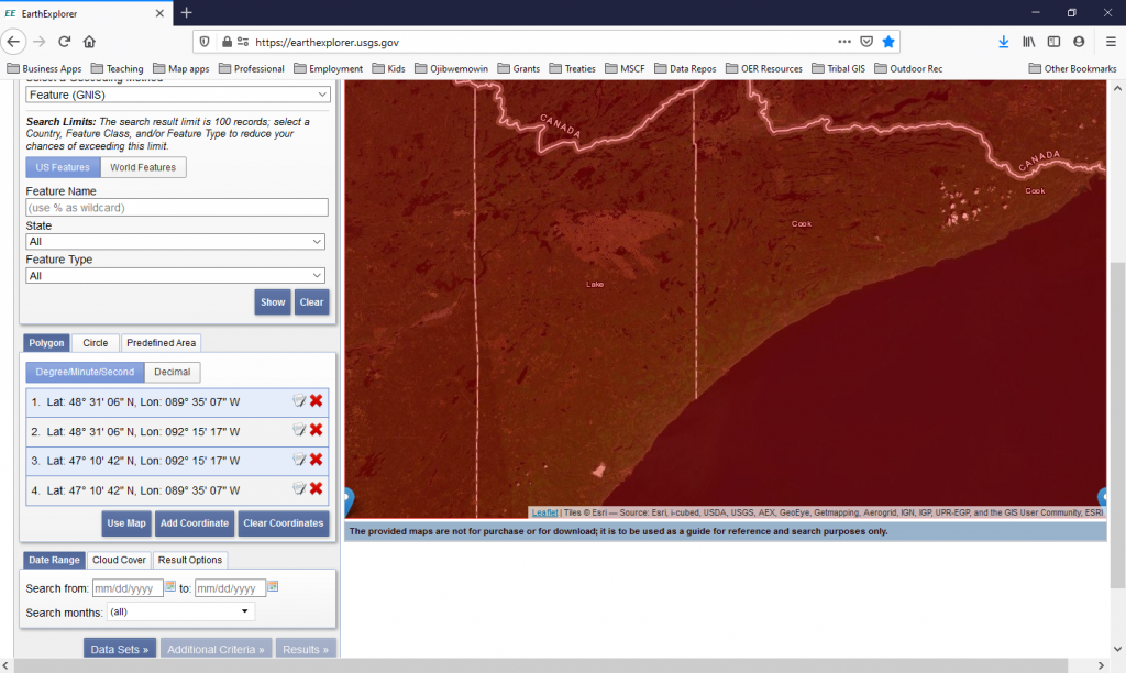
8. Optional: If you have a certain date range you want to search for imagery from, enter it under the “Date Range” tab.

9. At the bottom of the left side panel, click the “Data Sets >>” button.

10. In the list of datasets in the left side panel, expand “Landsat”, then expand “Landsat Collection 2 Level-2”, then check the checkbox for “Landsat 8 OLI/TIRS C2 L2”. (Note: If you want imagery from earlier than 2013, you must select an earlier Landsat mission; see the Landsat Mission Timeline to inform your selection).

How do you know what Landsat data to use?

Landsat imagery data is organized into a tiered structure that can be confusing.

The two Landsat Collections are series of Landsat imagery that each contain the same archive of images (called scenes), but georeferenced slightly differently (see Section 2.6 for more on georeferencing raster data). Collection 2 came about as an effort to reprocess old Landsat imagery to a higher standard of positional accuracy, and will ultimately replace Collection 1 for new data. Collection 2 data is currently available for Landsats 4-8, while Collection 1 data is available for all Landsat missions as of this writing.

Landsat Levels represent the amount and type of processing the imagery has undergone.

Level-1 imagery has just been georeferenced; it contains the original spectral reflectance values recorded by the satellite sensor, and can be placed in its correct geographic position by GIS software.

Level-2 data shows surface reflectance and surface temperature, or the amount of electromagnetic radiation of certain wavelengths that bounces off of the Earth’s surface (reflectance measures visible and near-infrared wavelengths, while temperature measures middle- and far-infrared wavelengths). Level-2 data has been processed to correct for signal distortions caused by gases and particulate matter in the atmosphere (Figure 2.36).

Level-3 datasets are derived from imagery that has been processed to show different biophysical properties of Earth’s surface, such as surface water extent, snow cover, burned areas, and evapotranspiration.

Landsat scenes are further divided into Tiers based on their quality. Tier 1 imagery is considered high-quality and suitable for analysis, while Tier 2 imagery has lower positional accuracy.

For more information on Landsat data, see the Landsat data products FAQ page here.

10. At the bottom of the left side panel, click the “Results >>” button.

Perception and Interpretation: The website takes a few moments to search the archive. Search results appear in the left side panel, ordered by date with the most recent imagery first. A thumbnail image, ID, Date Acquired, Path, and Row is listed for each Landsat scene. A row of buttons below the information for each scene allows you to show the scene’s footprint on the map, show a preview of the scene (browse overlay) on the map, compare browse, show metadata and browse, download the scene, add the scene to bulk download, and exclude the scene from the search results.

11. In the search results, click the Footprint button below each scene on and off to view the area covered by the scene.

12. When you find a scene that covers your area of interest, click the Show Browse Overlay button to view a preview of the image and evaluate its level of cloud cover.

13. Continue viewing results until you find a scene you are satisfied with. Note the date the scene was acquired.

14. Click the Download Options button for your selected scene, then click the “Product Options” button.

15. Near the top of the Product Download Options window, click the gray download button for the Product Bundle. When prompted, save the file to your downloads folder.

Add Landsat image bands to an ArcGIS Pro project

Once the Landsat scene has downloaded, it must be extracted from its .tar archive file to a project folder before it can be used. This extraction requires a file archiver program such as 7-Zip, which is free and open-source. Each .tif file that ends in B and a number is a raster dataset containing the sensor data for one image band, or set of electromagnetic wavelengths recorded by the sensor. The bands can be added to the map and displayed as individual layers of grayscale imagery.

Action Sequence

16. Open ArcGIS Pro. If you already have a project that you want to add the Landsat imagery to, open it; if not, create a new map project.

17. From the Windows Search Bar or Start Menu, open 7-Zip File Manager. If you can’t find 7-Zip, download it here and install it.

18. If the file path is not set to the Downloads folder, navigate to your Downloads folder in the main area of the window.

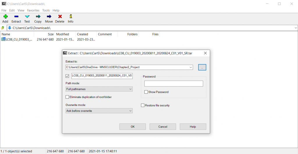
19. Click on the Landsat .tar archive file to select it, then click the “Extract” button (which looks like a blue minus sign).

20. In the Extract window, under “Extract to:”, click the “…” button to the right of the file path dropdown (Figure 2.37).

21. In the Browse For Folder window, navigate to your ArcGIS Pro project folder, then click OK.

22. In the Extract window, click OK.

23. Close 7-Zip and return to your ArcGIS Pro project.

23. In the Catalog Pane, expand the Folders item, refresh the project folder (right click on it, then click “Refresh”), and expand it to verify that it now contains a folder with the Landsat imagery.

Perception and Interpretation: If you see a folder with the Landsat scene ID, it indicates that the archive was successfully extracted into your project folder. If you do not see the Landsat folder, you may still need to refresh the project folder in the Catalog pane, or you may have extracted the imagery to another location on your computer. The Landsat folder contains a .xml file and several .tif files with the scene ID as the first part of the filename.

24. Set the map’s projection to the UTM zone for the part of the world your Landsat imagery covers. An interactive map of UTM zones is available here. See Section 1.6, Steps 4-8 for directions on how to change the map projection.

25. Add each of the Landsat .tif files that end in “B” and a number to the map, either by dragging them over from the Catalog Pane or using the Add Data button in the Map ribbon tab.

Perception and Interpretation: Each raster file takes a few moments to load onto the map while ArcGIS Pro builds pyramids. Image pyramids speed up future loading and processing of the raster file.

Composite imagery bands

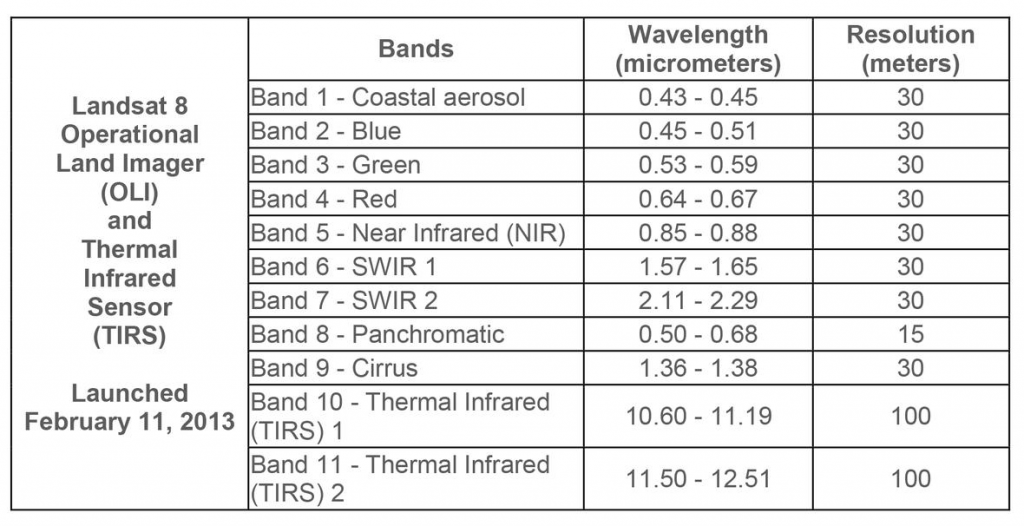
Each band of a Landsat scene includes data for a particular range of electromagnetic wavelengths. Some of these wavelength ranges are colors within the visible part of the electromagnetic spectrum, and some lie just beyond human vision, in the near infrared part of the spectrum. The wavelength ranges of each band are listed for all Landsat sensors here. Below is the list of bands for Landsat 8 (Figure 2.38):

Because each band’s .tif raster only contains a single set of reflectance values, it can only be rendered on the map in grayscale (or another assigned color gradient). In order to view the imagery in color, you must composite the image bands into a single layer. You can then choose three of the bands to assign to color channels of the display—one each for the red, green, and blue channels.

Action Sequence

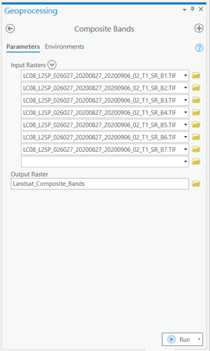
26. In the Analysis ribbon tab, click the “Tools” button to open the Geoprocessing pane.

27. In the Geoprocessing pane, search for and open the Composite Bands tool.

28. In the Geoprocessing pane, next to “Input Rasters”, click the down arrow and check the boxes for all of the Landsat band files in order from top to bottom, then click “Add”. (Note: The order is important; band numbers should begin at 1 and go up as shown in Figure 2.39).

29. Under “Output Raster”, browse to the project geodatabase and name the output raster “Landsat_Composite_Bands”.

30. At the bottom of the Geoprocessing pane, click the “Run” button (Figure 2.39).

Perception and Interpretation: The composite operation may take a few minutes to run. When finished, the Landsat_Composite_Bands layer is added to the Contents pane above the other raster layers, and displayed on the map as a color image. The image color is not true color and needs to be adjusted.

Create Color Imagery

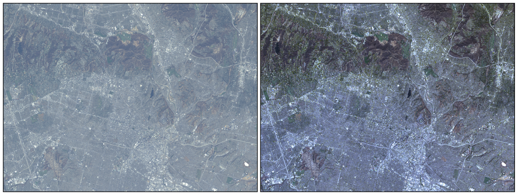
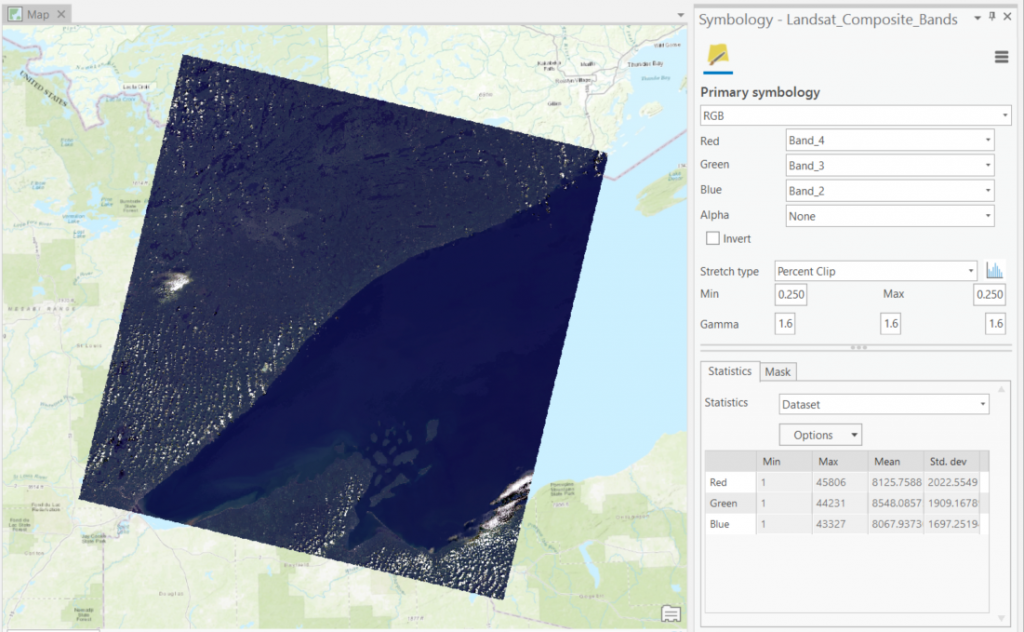
The composite layer can be displayed as true-color or false-color imagery by assigning different Landsat bands to different color channels. True-color imagery assigns the red band to the red color channel, the green band to the green color channel, and the blue band to the blue color channel. The result is color imagery that appears close to what you would see with the naked eye if you were looking down at the surface from the position of the sensor.

31. Remove all of the individual Landsat band layers from the Contents pane, leaving the composite layer as the only raster layer above the basemap.

32. Right-click on the Landsat_Composite_Bands layer name, then click “Symbology” to open the Symbology pane.

33. Based on the band numbers you wrote down in Teachback 15, in the Symbology pane, change the “Red” dropdown to the red band number, the “Green” dropdown to the green band number, and the “Blue” dropdown to the blue band number (Figure 2.40).

Perception and Interpretation: Changing each color channel dropdown’s band number changes the color of the image. When each band is correctly matched to its color channel, the image should appear approximately true color, though it may still look tinted or washed out and need adjustment. If the color of the image appears very wrong, the Landsat band rasters may not have been added to the composite in the correct order, or the wrong files may have been added (see the note in Step 28).

Adjust the image appearance

Assigning bands to channels in the right order makes the image appear closer to true color, but it likely still needs adjusting to look vibrant and realistic rather than tinted and washed out. This adjustment can be made using the tools in the Appearance tab and in the Symbology pane. These tools give you control over the image brightness, contrast, and gamma. Increasing brightness increases the values of pixels in the image bands. Increasing contrast increases the difference between pixel values by increasing high values and decreasing low values. An image histogram divides the full range of pixel values in the raster image into bins and shows how many pixels are assigned to each bin. A histogram stretch controls the direction and magnitude of the contrast adjustment by designating a certain number or percentage of high-value pixels to designate as the maximum pixel value and a certain number or percentage of low-value pixels to designate as the minimum value (usually zero), then reassigning other values in a relative way to fill the space in between. Decreasing gamma increases contrast in low values and decreases contrast in high values to compensate for differences between digital imagery and human light perception.

Action Sequence

33. Zoom in on part of the image with a diversity of land cover to see as much detail as possible without the image appearing fuzzy or pixelated.

34. In the Symbology pane, to the right of the “Stretch type” dropdown, click the Histogram button (which looks like a blue histogram) to display image histograms for the red, green, and blue channels.

35. With the Landsat_Composite_Bands layer selected in the Contents pane, click on the Appearance ribbon tab.

36. In the Appearance ribbon tab, click the “Stretch Type” dropdown, and select “None”.

Perception and Interpretation: The appearance of the image becomes duller and more washed out. In the Symbology pane, the vertical dashed lines, which represent the boundaries of the histogram stretch, move to the edges of each histogram. The colored histogram bars become closer together, appearing similar to but offset from the gray histogram bars.

37. Use the “Stretch Type” dropdown in the Appearance ribbon to assign different stretch types.

38. After experimenting with each stretch type, choose a stretch type that makes the image appear closest to the true color of the landscape.

39. Try adjusting each color channel’s image stretch manually by moving the sliders under the vertical dashed lines. Place each color channel’s boundary lines close to the gray histogram on either side of it, stretching the colored bars across as much of the graph as possible (Figure 2.41).

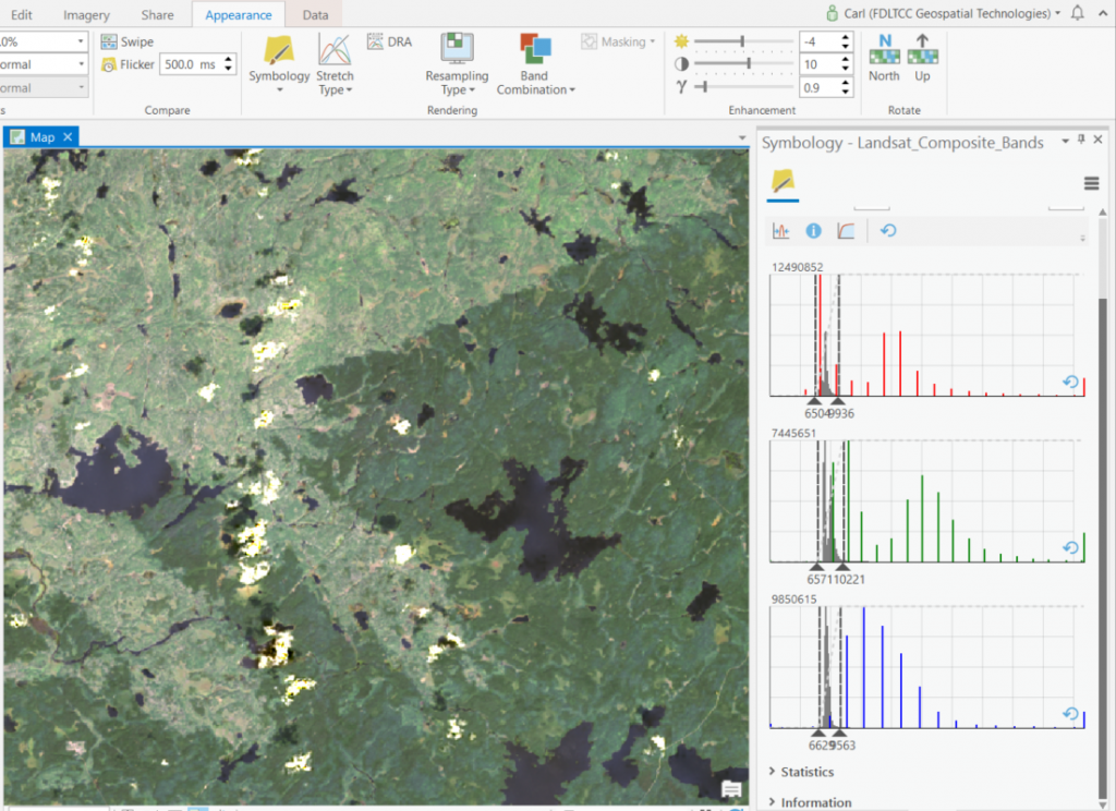
40. In the Appearance ribbon tab, in the Enhancement group, experiment with changing the brightness, contrast, and gamma sliders or values and observe the resulting change in the image appearance.

41. When satisfied that the image appearance is as crisp, detailed, and color-realistic as you can make it, save the project.

Create a false-color image

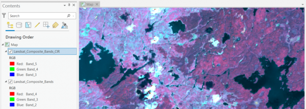
False-color imagery uses different band combinations that may be useful for emphasizing landscape features that are harder to see in true color imagery. For example, color infrared imagery assigns a near infrared band to the red channel, red band to the green channel, and green band to the blue channel. This band combination makes healthy growing vegetation stand out in bright reds and pinks, while areas with little or dormant vegetation appear blue or gray, and water appears very dark. Other band combinations can be used to emphasize soil moisture, fire damage, and various other landscape phenomena.

42. In the Contents pane, copy and paste the Landsat_Composite_Bands layer to duplicate it on the map.

43. Rename the duplicate layer “Landsat_Composite_Bands_CIR” (“CIR” stands for “Color Infrared”).

44. In the Symbology pane for the Landsat_Composite_Bands_CIR layer, reassign the bands so the Red channel is assigned the first near infrared image band, the Green channel is assigned the red band, and the Red channel is assigned the blue band. Refer to your answer to Teachback 15 for the band numbers of these bands.

45. Readjust the image stretch and enhancements as needed to reveal as much detail as possible in the color infrared image (Figure 2.42).