Excel Chap 1 – Spreadsheet Basics
- What is a Spreadsheet?
- Entering, Selecting and Inserting Data
- Manipulating Sheets
- Formatting Worksheets
- Creating Formulas to Perform Calculations
- Copying and Pasting Formulas
- Adding Basic Functions to Formulas
- Inserting Headers and Footers
- Adjusting the Page Layout and Preparing to Print
What is a Spreadsheet?
A spreadsheet is a collection of data that is organized into rows and columns. Microsoft® Excel is a spreadsheet application used to store and analyze quantitative data. An Excel file is called a workbook, and it is saved with an .xlsx extension. A workbook file consists of one or more worksheets which consists of many columns and rows. Columns are the vertical part of a worksheet grid identified by letters. Rows are the horizontal part of a worksheet grid identified by numbers. The intersection of a row and column is called a cell. Each cell can store a single item of data. The data can contain text, numbers, formulas, and/or functions. Clicking a cell with the mouse pointer will make the selected cell the active cell. The active cell’s contents are displayed in the formula bar.
Typical uses for Excel include:
- Accounting reports (Balance Sheets, Income Statements, etc)
- Budgets
- Calendars
- Checklists and task lists
- Contact/Address lists
- Expense tracking
- Inventory control
- Invoices
- Mortgage and other financial calculations
- Operational statistics
- Sales price lists, forecasts and analysis
Entering Data
 Excel is great tool for generating useful information from data. However, the data has to be entered before it can be analyzed and manipulated. There are numerous types of data, and numerous ways to streamline data entry. As data is typed, it appears in the active cell and in the formula bar. Pressing the Enter key will complete data entry and make the next cell in the column the
 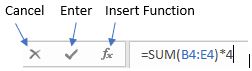 active cell. If moving to the next cell after completing data entry is not the desired outcome, try clicking the Enter check mark in the formula bar. The data will be entered, but the active cell remains the current cell. Pressing the Esc key before completing data entry will cancel data entry and restore the original cell contents.
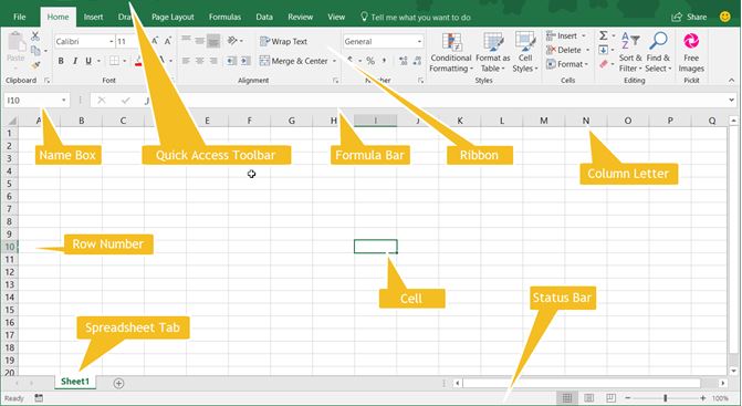
Streamlining data entry in Excel can be accomplished using several different features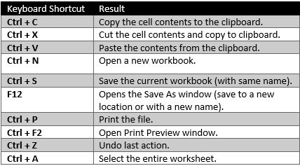 including keyboard shortcuts and Automatic Completion. Keyboard shortcuts allow rapid navigation in a worksheet without having to use the mouse. There are hundreds of keyboard shortcuts available in Excel and many are also available in other Microsoft Office applications. A few keyboard equivalents are illustrated at right, but for more examples, use the shortcut F1 to open the Help pane, and type keyboard shortcuts in the Excel Help field.
When entering data into a sheet that contains a lot of duplicates, Excel uses the 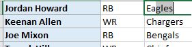 Automatic Completion feature to speed up data entry. After typing a couple of characters, Excel guesses how to fill the rest of the cell based on data previously entered in the cells above. To accept the suggestion (in highlighted text), press Enter, or alternatively, continue typing to replace the automatic entry.
Selecting Data
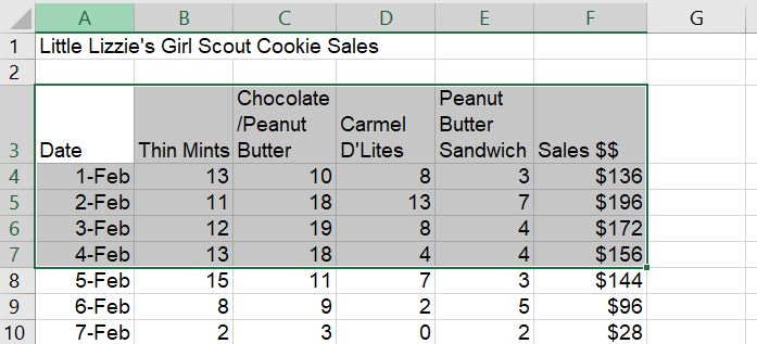
After entering data, a common practice is to begin formatting the data. However, before a user can format the data, they must first select the data. Selecting data has multiple techniques based on user intent. Clicking on a single cell makes that cell the active cell. The cell reference appears in the Name box to the left of the formula bar. To select an entire column of data, just click the column letter heading. To select an entire row, click the row number heading. If a user wants to select several cells adjacent to each other, this would be considered selecting contiguous cells. Clicking the middle of the cell and dragging horizontally or vertically will select a contiguous range of cells. Another way to select a contiguous range of sequential cells is to click the first cell, hold down the Shift key, and click the last cell in the range. For example, clicking cell A3, and then holding down the Shift key and selecting F7 would select all of the cells from A3 through F7. The range reference would be written as A3:F7.
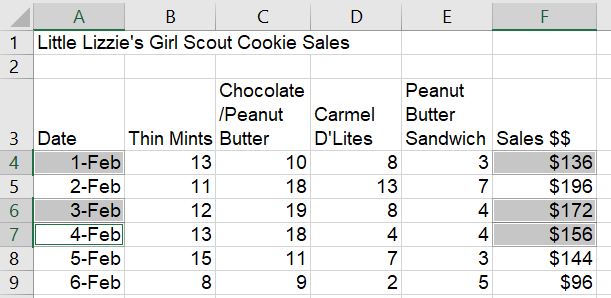
Selecting a non-contiguous range of cells requires the use of the Ctrl key. To select non-contiguous cells, click the first cell, hold down the Ctrl key, and click each additional cell. This practice is sometimes referred to as “cherry-picking” cells. In the example below, the selected range of cells are A4,A6,A7,F4,F6,F7. This practice can be used for selecting non-adjacent rows or columns as well.
To select the entire worksheet, click the triangle box located to the left of column A and above row 1, or by pressing the keyboard shortcut: Ctrl+A.
Inserting Data
It is usually easy to add data to an existing worksheet, because Excel has seemingly unlimited columns and rows of cells. (There are limits, but this is not Jeopardy!) Nonetheless, sometimes it is necessary to insert a column or row into the middle of an  existing range of cells. To insert a new column, select the column heading to the right of where you want the new column to appear, and click the top-half of the Insert button from the Home tab. Alternatively, just right-click the column heading to the right of the destination, and choose Insert from the Context Menu. Deleting columns is very similar. Whichever column(s) that are selected will be deleted if using the Delete button instead of the Insert button. Inserting and deleting rows is also very similar. Selecting the row below the intended new row and either choosing Insert from the ribbon or from the Context Menu will create a new row above the selection. For example, right-clicking row 10, and choosing Insert from the Context Menu will create a new, blank row 10, and all existing data will move down one row.
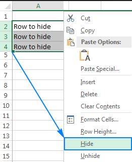
Using the right-click method is a little faster than clicking the worksheet and then clicking the ribbon, as the shortcut menu avoids the need to move the mouse to the ribbon. The Context Menu, also known as Shortcut Menu, provides added functionality by offering actions that can be taken with the selected item. In addition to inserting and deleting, formatting column widths and row heights, as well as hiding and unhiding columns and rows are options from the Context Menu. Adjusting the column width is a common action since excessively wide columns prohibit efficient worksheet printing. Therefore, it is often preferable to widen a column width by double-clicking the boundary bar that separates the column heading letters. This is known as 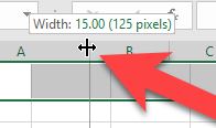 auto-fitting the column width since the column will resize its width to be just wide enough to display the longest data contained in that column. Clicking and dragging the double-arrow pointer to the left or right allows users to manually adjust the column width.
Manipulating Sheets
An Excel workbook consists of one or more worksheets. Much like a binder can have multiple sections of sheets divided by colorful tabs, an Excel workbook can multiple 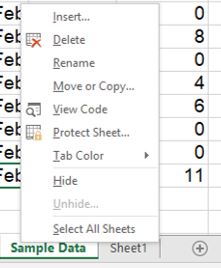 sheets that can be re-arranged, colored and renamed to fit individual organization plans. Inserting and deleting worksheets is similar to the inserting of columns and rows. In addition to using the Insert or Delete buttons from the ribbon, right-clicking an existing sheet tab will produce a Context Menu with a plethora of options.
Just as inserting a new column will add the column to the left of the selected column, the newly inserted worksheet will appear to the left of the selected sheet tab. Options exist to insert a blank worksheet or a new sheet based off of an existing template. Clicking and dragging sheet tabs are easy method to rearrange the order of sheets. However, the Move or Copy… command offers the opportunity to move or place a duplicate sheet within an existing, open workbook. Adding tab colors and the Rename option can help organize sheets to user-specific criteria. Sheets can also be hidden and unhidden. If it is necessary to prevent others from unhiding sheets, the workbook can be protected with a password to be able to modify the sheets. The tab scrolling buttons to the left of the sheet tabs are enabled when too many sheets exist to be displayed above the status bar. To quickly add a new, blank sheet to the workbook, click the plus button ![]() to the right of the sheet tabs.
to the right of the sheet tabs.
Formatting Worksheets
Formatting data generally makes it easier to comprehend, and more attractive. The goal of formatting a business spreadsheet should be to make it look professional, accurate, and understandable. Options to format worksheet data depends a lot on the type of data. Formatting text in Excel is very similar to formatting text in Word. Using the Font and Alignment group icons on the Home tab of the ribbon, users can manually format all of the data in a cell or in a range of cells. Changing default formats includes things like changing the font color, style, size, text alignment in a cell, or apply formatting effects – all in an effort to make the data appear more visible.
Excel’s tabular layout (organized into labeled columns and numbered rows) sometimes limits the amount of data that can be efficiently displayed. Using the Alignment group 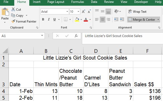 options can help format data to make it appear as much like a word processed report as possible. In the screenshot above, two Excel-unique formatting features help make the data more readable. In row 1, the text has been merged and centered across cells A1:F1. This required the cell range A1:F1 be selected before clicking the Merge & Center button from the Alignment group. This is very popular for worksheet titles. If the wrong cell range was selected and the Merge & Center is not effective, the user must re-select the Merge & Center button to unmerge the data, so the correct range can be selected before again clicking the Merge & Center button.
Another popular Excel text-formatting feature illustrated above is the Wrap Text tool, which will prevent text from being truncated by wrapping the text into multiple rows within the same cell. If a cell has a lot of text, the data will overlap into the next cell to the right of the active cell. However, if the adjacent cell already has data, the text will be truncated (cut-off) without applying this feature. Cells C3:E3 in the above screenshot each have the Wrap Text feature applied.
While Excel has some pretty useful text-formatting functionality, the majority of data entered into Excel is usually numerical data. Therefore, utilizing Excel’s number formats effectively is crucial to make the worksheet as professional as possible. Professional formatting relies a lot on consistent formatting. Therefore, using the Format Painter tool (introduced in the Word chapters) and workbook themes are very helpful to maintain that consistency. Changing the existing theme will dynamically update the appearance of all worksheets in a workbook by modifying the fonts, styles, colors and/or effects.
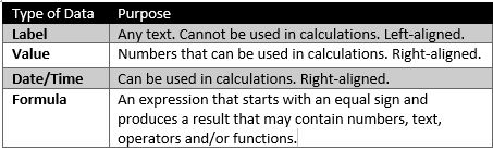
Applying the correct cell format to numerical data is more than just style – it is substance too, because applying the wrong format can impact how other, related cell results are interpreted. The following graphic describes some of the more popular number formats. In addition to the examples provided, there are also other formats, including date & time values, which can be accessed by clicking the Number Format drop-down list.
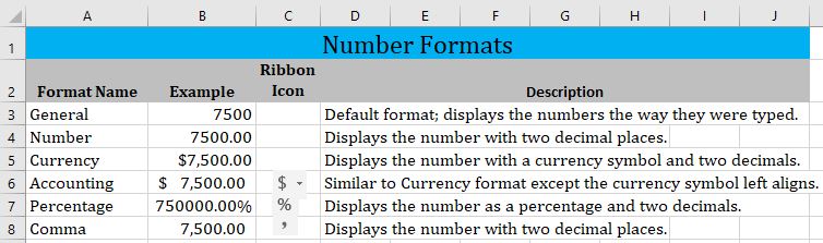
Changing the number of decimals displayed can be manipulated by the Increase Decimal and Decrease Decimal buttons in the Number group. The displayed value could change to a rounded value, however, the actual value stored in the cell has not changed unless a ROUND function has been applied. Formatting only affects how the value is displayed. Applying formats can result in number signs (#####) being displayed in a cell. This is not an error, but an indication that the cell width is not wide enough to display the formatted number.
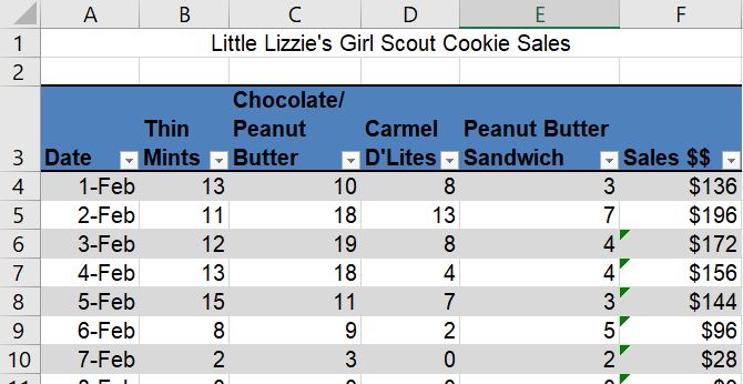
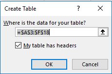
Excel data can also be formatted as a table. A table is a collection of related data, organized into a tabular layout of rows and columns, that can be manipulated via sorting, filtering and formulas. To create a table, select the data and click Insert > Table from the ribbon to open the Create Table dialog window.
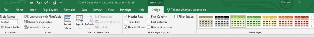
Applying a table style will format the table with a predefined set of special table properties that includes options to define a header row or total row, and to band the row and/or columns to make the data easier to read. The filter buttons can also be removed. If the table functionality is no longer desired, click the Convert to Range option in the Tools group of the Design tab to convert the table to a normal range.
There are many additional formatting tools available within Excel, but it is important to consider that sometimes, less is more! Too much formatting can be overkill and reduce the readability of a worksheet. Try to limit the use of multiple colors, fonts, and background colors/graphics. Format with a design purpose, not to entertain, and don’t forget to use the Spell Check tool (F7) to proof your workbook before printing or sharing!
Creating Formulas to Perform Calculations
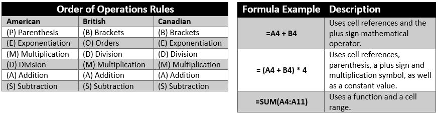
Perhaps the biggest benefit of using Excel is its ability to create formulas that, when written correctly, can dynamically update when predecessor data is updated. Formulas are mathematical calculations using data in the existing workbook to calculate new values. All formulas in Excel must begin with an equal sign (=), and can contain cell references, ranges of cell references, arithmetic operators, and constants as part of the formula’s syntax. Calculations in Excel follow normal math rules as it pertains to the order of operations rule. There are mnemonics available in various dialects to help decipher the order. The following graphics illustrate the order of operations rules and different formula syntax examples:
Formulas typically reference values stored in other cells. For example, in the Accounting equation: Assets = Liabilities + Owner’s Equity, one could calculate the Owner’s Equity using a formula. Assume that the value for Total Assets resides in cell D30, and the value for Total Liabilities resides in D60. The formula for Owner’s Equity in D65 using cell references would be =D30-D60. Using cell references is advantageous because if any of the cells that generate either the Total Assets or Total Liabilities is changed, the formulas in D30, D60 and D65 will also get updated. Another advantage is when a cell containing a formula is copied to another location, the formula will dynamically update to the new location’s reference information. This is called Relative Cell Referencing. If the formulas in column D are copied to column E, the new formula for Owner’s Equity in column E will be =E30-E60. Additionally, if rows are added or deleted in the range that the Total formulas reference, the formula will automatically update to the new formula range.
Entering the syntax for a formula can be accomplished through typing the formula components, using a pointing technique or a combination of both. The pointing method can help avoid typing errors. In the Owner’s Equity example, the user would start by typing the equal sign, and then instead of typing D30, just click on D30. Continue by pressing the minus sign, and then click on cell D60, and the click the Enter check mark on the formula bar. Using the point method is even more practical when defining large cell ranges in formulas. Just make sure not to reference the active cell in the formula. This will likely create a circular reference error, which is a formula in a cell that directly or indirectly refers to its own cell.
Copying and Pasting Formulas
![]() Data in Excel can be cut, copied and pasted using similar shortcut menu options, keyboard equivalents, and ribbon icon commands as seen in Microsoft Word. Following operating system file management principles, moving data is synonymous with using the “Cut” and “Paste” commands, while duplicating data is the same as using the “Copy” and “Paste” commands. Other terminology that should be recognized is “source”, which is the cell or range to be moved or duplicated, and “destination”, which is the upper-left cell in a worksheet where the data is to be pasted.
Data in Excel can be cut, copied and pasted using similar shortcut menu options, keyboard equivalents, and ribbon icon commands as seen in Microsoft Word. Following operating system file management principles, moving data is synonymous with using the “Cut” and “Paste” commands, while duplicating data is the same as using the “Copy” and “Paste” commands. Other terminology that should be recognized is “source”, which is the cell or range to be moved or duplicated, and “destination”, which is the upper-left cell in a worksheet where the data is to be pasted.
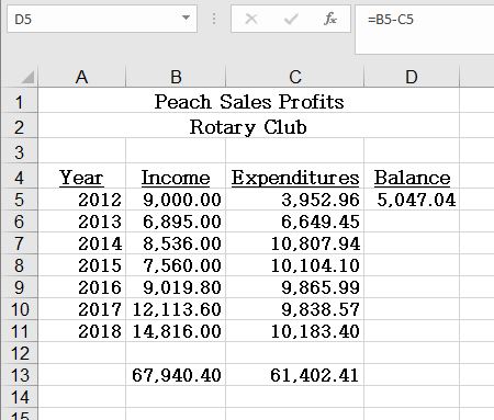
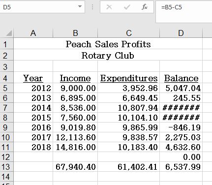
Copying and pasting formulas contain cell references is a very powerful feature, and to expedite this process, Excel has a nifty feature called AutoFill. The AutoFill procedure utilizes the fill handle, which is the solid, green square in the lower-right corner of the active cell or cell range. Clicking and dragging the fill handle to adjacent cells (horizontally or vertically) will copy and paste the contents and update the destination cells with relative cell references or sequential data aligned with built-in Custom Lists. This should save significant time, and likely improve accuracy, and AutoFill has many uses. 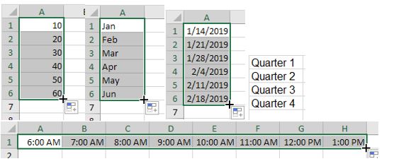 Not only can AutoFill copy formulas, but it also be used to complete lists that have a recognizable pattern. It is helpful to select the source cells that demonstrate a pattern, then hover the mouse pointer over fill handle. The mouse pointer will change from the default pointer icon to a thin, black plus sign. The patterns can be numbers, dates, months, days of the week, etc. If AutoFill incorrectly guesses the series pattern, the AutoFill Options icon is available to change the paste actions. In the screenshots below, the fill handle in cell D5 will by copied to cells D6:D13. The results shown in the second screenshot will update the formula from D5 with relative cell references to rows 6:13. What is happening in cells D7:D8?
Practice 5: Test Scores
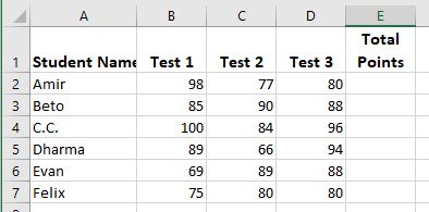
- In a new Excel workbook, enter the following data:
- Make sure to apply bold formatting to row 1, and text wrapping to cell E1.
- Format the data as a table with a header row and banded rows, but no Filter buttons.
- Apply the Facet theme.
- Ensure that cell E1 has the text wrapping format applied and then resize the column width of column E to be 7 points wide and the height of row 1 to 36 points.
- AutoFit columns B, C & D.
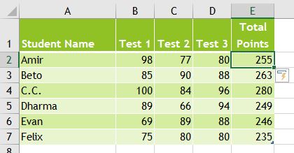
- In cell E2, enter the following formula: =B2+C2+D2 and click Enter. Your worksheet should look like the screenshot at right. Notice that Excel automatically filled in formulas for the rest of column E cells using relative cell references! If this action is unwanted, click the lightning icon, and choose to Undo the Calculated Column.
- Press F12 to invoke the Save As command and save the file as Test Scores.xlsx.
Adding Basic Functions to Formulas
Excel contains over 400 built-in functions that can be included in a formula to perform common calculations. A function performs a calculation on data called arguments to compute a result. Arguments are variables or values the function requires and are contained within parenthesis, and usually consist of cell references, but can also contain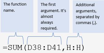 constants, text, cell ranges, and even other functions! The syntax of a formula using a function is: function name(argument1, argument2, etc.) Functions can be typed with the help of a ScreenTip, or added from the Insert Function window, which can be opened by clicking the
 ![]() symbol found at the left of the formula bar, or at the left side of the Function Library found in the Formulas tab of the ribbon.
symbol found at the left of the formula bar, or at the left side of the Function Library found in the Formulas tab of the ribbon. 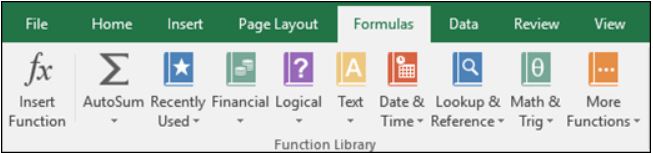
The most popular functions are also the easiest to comprehend, which might be correlated! Some of these most popular functions are easily accessible from the AutoSum button in the Editing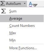 group on the Home tab of the ribbon. Look for the Greek sigma symbol. This feature is invaluable when it comes to entering functions, especially for common calculations computed via the SUM, COUNT, AVERAGE, MAX or MIN functions. There are multiple ways to utilize AutoSum, but the following procedure is probably the simplest. In the screenshot below, assume the desire is to total the number of boxes of Thin Mints cookies were sold the first 15 days of February. Make B19 the active cell (the destination cell), then click the AutoSum button. The defaulting SUM option will be inserted into the formula bar with a defaulting cell range (the source cells) inside parenthesis. The cell range that defaults appears on screen with a scrolling marquee surrounding the cell range. This range is usually correct, but not always. If Excel chooses the wrong range, simply type in the cell range, or use the mouse to re-select the correct range (pointing method), and then click the Enter check mark.
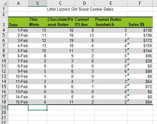
The formula that defaults should be =SUM(B4:B18). Once this formula is submitted, the result, 97 will display. The intent of the SUM function is pretty self-explanatory. The AVERAGE function takes the SUM function one step further by dividing the sum of the values by the number of cells in the range. The MIN and MAX functions are used to find the smallest and largest values in a range of cells. These can be useful to identify outlier data that might skew the results. Each of these functions ignore cells that contain text or are empty. Alternatively, the COUNT function totals the number of cells that contain values. If a cell contains the value 0 (zero), it will be counted. However, if the cell is blank or contains the text zero, the cell will not be counted. This function is useful for determining the number of people who mark a checkbox in an Employee roster. For example, how many employees identify as a Veteran? Those who don’t, wouldn’t have a value, and therefore, would not be counted. If the desire if to count all cells that contain any data – use the COUNTA function.
Inserting Headers and Footers
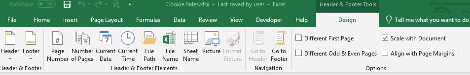
In Excel, headers and footers are lines of data that print at the top (header) and bottom (footer) of each page in a worksheet to help identify printouts. Headers and footers can contain descriptive text, graphics, and/or fields, such as titles, dates, or page numbers. Header and footer information does not display in Normal view, so to edit a header or footer, click Insert > Header & Footer to open the sheet in Page Layout view, and activate the Header & Footer Tools contextual tab on the ribbon. There are left, center and right sections for both the header and footer areas.
Users have the option to use one or more of the many built-in headers and footers, or they can click any of the buttons in the Header & Footer Elements group on the Header & Footer Tools Design toolbar to create custom fields.
Command buttons in the Header & Footer Elements group include:
-
-
- Page Number: Click this button to insert the
&[Page]code that puts in the current page number. - Number of Pages: Click this button to insert the
&[Pages]code that puts in the total number of pages. - Current Date: Click this button to insert the
&[Date]code that puts in the current date. - Current Time: Click this button to insert the
&[Time]code that puts in the current time. - File Path: Click this button to insert the
&[Path]&[File]codes that put in the directory path along with the name of the workbook file. - File Name: Click this button to insert the
&[File]code that puts in the name of the workbook file. - Sheet Name: Click this button to insert the
&[Tab]code that puts in the name of the worksheet as shown on the sheet tab. - Picture: Click this button to insert the
&[Picture]code that inserts the image that you select from the Insert Picture dialog box that enables you to select a local image (using the From File option) or download one from an online source using a Bing Image Search. - Format Picture: Click this button to apply the formatting that you choose from the Format Picture dialog box to the
&[Picture]code that you enter with the Insert Picture button without adding any code of its own.
- Page Number: Click this button to insert the
-
The following screenshot illustrates fields in each section of the header. The Page Number and Number of Pages fields are in the left section. Manually entered text is in the center section, and finally, the Current Time and Current Date fields are being inserted into the right section. 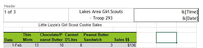
To create a custom header or custom footer, click the Launcher icon in the Page Setup group of the Page Layout ribbon to open the Page Setup window. Next, click the Header/Footer tab, and then choose to open either the Custom Header… or Custom Footer… buttons. 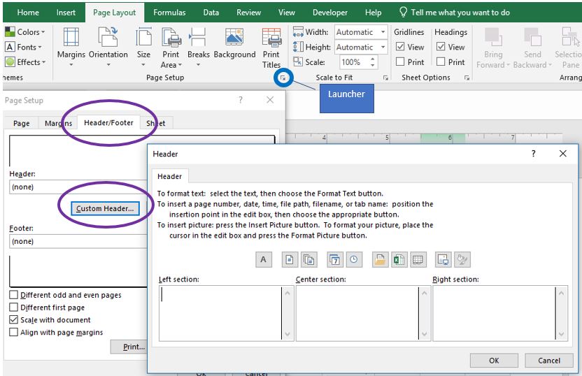
Four checkboxes appear at the bottom of the “Header/Footer” tab, and in the Options group of the Design tab of the ribbon. To remove headers and footers from the first printed page, select the Different First Page check box. To specify that the headers and footers on odd-numbered pages should differ from those on even-numbered pages, select the Different Odd & Even Pages check box. These options are similar to those in Microsoft Word. The other two options are unique to Excel. To specify whether the headers and footers should use the same font size and scaling as the worksheet, select the Scale with Document check box. To make sure the header or footer margin is aligned with the left and right margins of the worksheet, select the Align with Page Margins check box.
Adjusting the Page Layout and Preparing to Print
The size of Excel workbooks tend to grow the more each worksheet is manipulated, typically by adding more columns and rows, and sometimes, more sheets. This added complexity makes physical output of Excel data somewhat challenging. Too many columns will result in the sheet not being able to be printed on one sheet of paper, and too many rows make make it difficult to interpret data on pages beyond the first page. Fortunately, the Page Layout tab can help fit the data on fewer sheets of paper and make each page easier to understand.
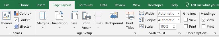
While themes can help modify the appearance of a spreadsheet’s colors and fonts, the other groups in the Page Layout tab can impact the arrangement of data, and streamline the readability of the output. Starting with the Page Setup group, Excel allows tremendous flexibility with the margins of each worksheet. For example, Narrow margins allow more data to fit on one page by reducing the amount of white space on the edges of the sheet. A quick and easy way to allow more columns to print on one sheet, is to change the orientation from the default Portrait, to Landscape, which allows more columns and fewer rows to print on one sheet. The effects of these Setup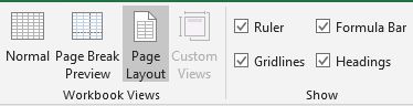 decisions can be more easily illustrated by switching from the default Normal workbook view to the Page Layout. The View tab also allows users to to enable/disable the Ruler, Formula Bar, and on-screen gridlines and headings.
If changing the margins and/or orientation is not resolving the issue of getting extra columns to print on the same page, an alternative could be changing the paper size. The default printer determines the paper sizes available from the Size drop-down list. To check the range of paper sizes that a printer can print on, consult the printer manual, or view the paper sizes that are currently set for the printer in the Print Setup dialog box. Some users have the option of printing to Legal (8.5″ x 14″) or even 11″ x 17″ (tabloid) printers, especially if commonly printing large worksheets.
A final, more drastic option to keep data from overlapping into multiple sheets, is to utilize the scaling feature. Using the Scale to Fit group from the Layout tab, a printed worksheet can be scaled by to modify the font size of printed output by either shrinking or enlarging the output. The options exist to scale the output to fit to 1 page wide (width) by 1 page tall (height). It might make sense to only modify the width, or by choosing a Scale percentage, which adjusts the overall sheet height and width proportionately. Keep in mind the needs of your audience. Too small of font might make the spreadsheet unreadable, and for certain audiences, the output might need to be scaled to a larger font than the editing view.
The Sheet Options group of the Layout tab provides two significant print features for basic Excel printing. These include the options to have gridlines and/or headings appear in printed output. By default, the options appear in the Viewing screen, but do not appear when printed. Without Headings, the output would be very difficult to explain to others, and gridlines, much like banded rows, make it easier for the eye to line up the intersections of rows and columns.
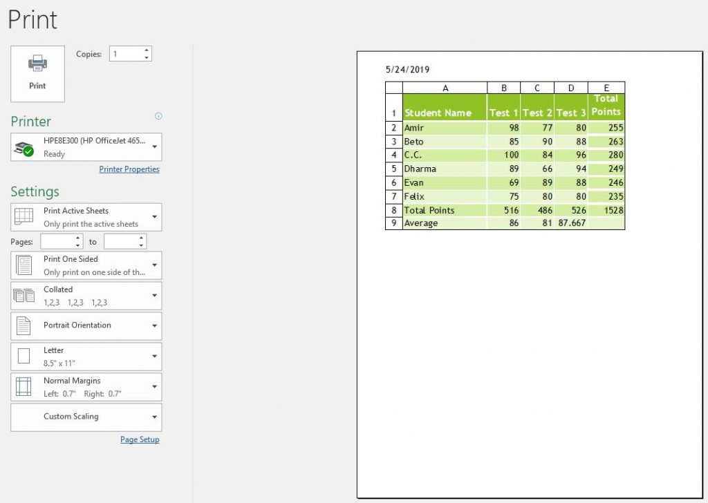
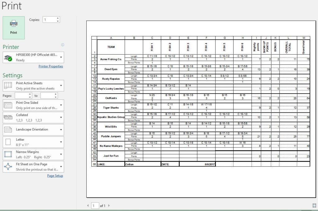
More advanced options exist for enhancing page layout and printing options by clicking the launcher button in each group. Additionally, several print settings can be adjusted in the Print Preview window. The sheet in the screenshot below is modified to print in landscape orientation with Narrow Margins and it is scaled to Fit on One Page. It also has headings included in the print output.
Practice 6: Test Scores, continued
- Open the Test Scores workbook previously saved.
- In the Table Tools Design tab, click the Convert to Range button remove the table functionality from the data. (Click Yes to the message)
- Type the labels: Total Points in cell A8 and Average in cell A9.
- In cell B8, click the AutoSum button to insert the SUM function. Accept the range that Excel proposes for the formula by clicking the Enter check mark on the formula bar. The formula should be: =SUM(B2:B7).
- With B8 as the active cell, use the fill handle to copy the formula to the destination cells C8:D8.
- In cell B9, enter a formula using the AVERAGE function without using the AutoSum functionality. Instead, use the Insert Function button to select the AVERAGE function, and enter the range B2:B7 as the arguments. NOTE: B8 should not be included in the range of argument cells. Use the fill handle to copy the formula to cells C9 and C10.
- In cell E2, double-click the fill handle. See what happens!
- Change the view to Page Layout.
- Add a header that includes the Current Date field from the Header & Footer Tools Design ribbon in the left side of the header.
- Ensure the Gridlines and Headings appear in printouts, scale the sheet to 150%, then view the file in Print Preview. Your worksheet should resemble the following:
- Save the file as TestScores2.xlsx.