
5 The Economics of Poverty
Caroline Krafft
What is poverty?
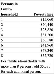
In the United States, poverty is measured relative to a federal poverty line (FPL) and depends on a family’s size. The basis of the poverty line is spending on food, updated for inflation, and multiplied by three. This basis is because, in 1955, when the data that determined the first poverty line were collected, food was one third of a family’s income. Box 5.1 discusses this historical basis of the poverty line. Table 5.1[1] shows the poverty lines in the U.S. as of 2024. A family of four, in 2024, would be considered “in poverty” if their income was below $31,200. Globally, similar poverty line construction is used in countries such as Egypt, which calculates a variety of poverty lines, also based off of food expenditure.[2]
The FPL is used to determine eligibility for a number of different anti-poverty programs in the U.S. There are a variety of critiques in using the FPL either to determine program eligibility or measure wellbeing. Recent estimates indicate that food is one-eighth, not one-third, of budgets, suggesting FPL provides a substantial underestimate of poverty. Some families may have additional expenses—such as child care needs—that are not accounted for in measuring poverty. Local variations in cost of living are not taken into account. The measure does not take into account taxes, which reduce disposable income. The measure also does not take into account non-cash public benefits, such as public housing, that may improve well-being substantially without changing (cash) income. Although alternative measures have been proposed, none have yet been implemented in the U.S.[3]
Box 5.1: Mollie Orshansky and the History of Poverty Lines in the U.S.[4]
Mollie Orshansky developed the modern system of measuring poverty for the U.S. At the time she developed the poverty lines, Orshansky was working for the Social Security Administration as a social science research analyst. She had training in economics and statistics and studied families’ budgets and spending. Orshansky calculated in 1955 that a family spent one third of their money on food. She then used the amount of money needed for an economy food plan as the basis for the poverty line, multiplying that amount by three to cover non-food expenses. Her initial work on poverty lines was published in a Social Security Bulletin in 1963. When President Lyndon Johnson declared a war on poverty in 1964, Orshansky played a key role in designing poverty thresholds that depended on family size and spending a third of the budget on food. Her poverty thresholds were made the official statistical definition of poverty in the U.S. in 1969.
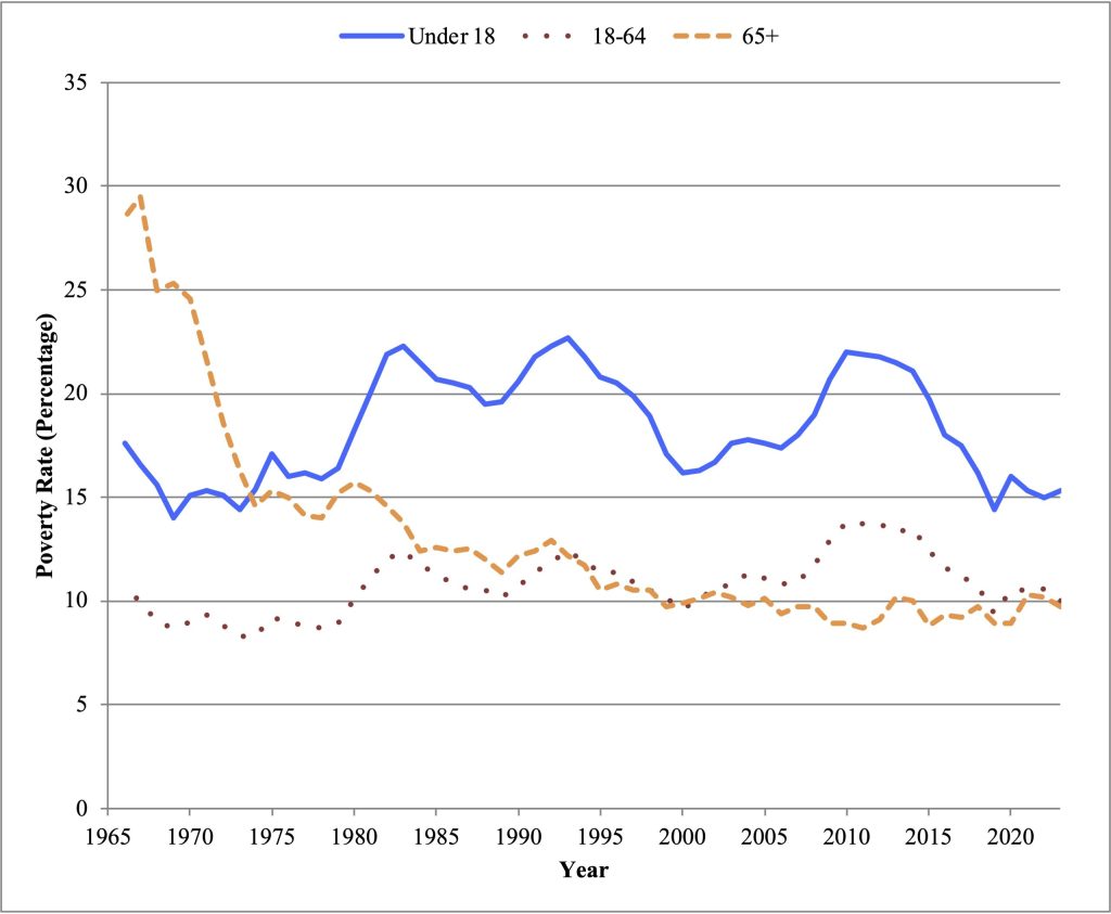
The progress the U.S. has made in fighting poverty over the past 50 years has been mixed. Figure 5.1[5] shows poverty rates from 1966, at the start of the “War on Poverty,” until 2023. Notably, the poverty rate for seniors (those 65+) has declined from a high of 29.5% in 1967 to just 9.7% in 2023. However, child poverty has fluctuated and is, as of 2023, the same (15.3%) that it was in 1970. Adult poverty has also fluctuated but is, as of 2023 (10.0%), at a similar level as in 1970 (9.0%). Notably, the “Great Recession,” the economic downturn the U.S. (and the global economy) experienced from 2007-2009 led to increases in poverty among children and adults, but not among seniors. The majority of seniors receive most of their income from Social Security,[6] which is not impacted by economic downturns. Social Security also played a key role in the decline in poverty among seniors in the late 1960s.[7]
Causes and models of poverty
On an economy-wide level, we know from Chapter 1 that a variety of factors, including the nation’s stock of capital, the quality of the labor force, the population, and technology play a critical role in a country’s level of development. When considering individuals or households, there is some overlap in the factors that cause poverty. Human capital and physical capital ownership (wealth) play a critical role in families’ poverty in the long run. There are also intergenerational aspects of poverty that are important to consider, as poverty tends to be transmitted across generations. Combatting poverty in the long run requires improving individuals’ and families’ levels of physical and human capital. In the short run, we can think about the causes of poverty as insufficient current resources. This section discusses models for understanding the causes of poverty in the short run and the long run.
The budget constraint: A short run model
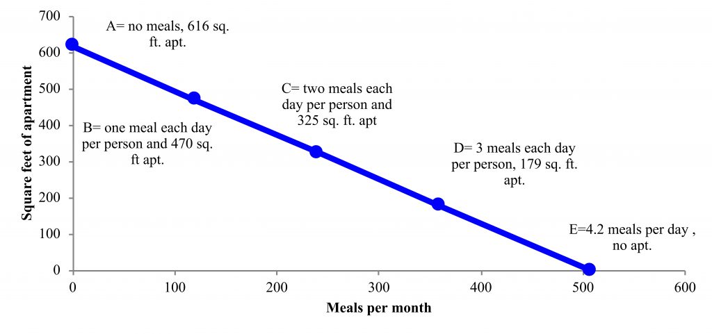
In the short run, we can model poverty using the idea of a budget constraint. The budget constraint shows the tradeoffs that a household faces, given its current resources. As with the production possibilities curve, the budget constraint simplifies the household’s spending choices into a model with two goods, such as housing and food, as in Figure 5.2. The units are the number of goods, determined given the price of different goods and the family’s income. Figure 5.2 is the budget constraint for a four-person household, with two parents and two children. One parent is working full time, forty hours a week, bringing home pay equivalent to the federal minimum wage of $7.25 per hour (we will ignore any taxes or subsidies for now). Over the course of a month, the family’s income is $1,232.50, and over the year, the family’s income is $14,790. They are in poverty (far below the FPL). Each month, the family spends only on meals, which cost $2.43 per meal (based on USDA estimates for a family of four with two young children and moderate costs),[8] and housing, renting an apartment. The cost for each square foot of apartment space is $2 (this cost is on the low end of major metropolitan rents).[9]
The (monthly) budget constraint shows the tradeoffs they face. They can, at point A, eat no meals, and have a 616 square foot (typical one bedroom) apartment. At point B, each person can eat one meal each day for the month, which with four people total, is 120 meals over the course of a 30-day month (this is equivalent to spending $292 on food, leaving $940 for housing, which pays for 470 square feet, a studio apartment). At point C, each person can eat two meals a day, but then the family can only afford 325 sq. feet of housing—a very small studio apartment. At point D, the family can eat 3 meals each day, but now can only afford 179 sq. ft. of housing—basically the size of a bedroom and a bathroom. At point E, the family has no housing, but can eat 4.2 meals per day. The slope of the budget constraint shows the tradeoffs the family faces. Given that a meal is $2.43 and a square foot of housing is $2, for each meal the family adds, they have to give up 1.2 square feet of housing. Likewise for each square foot of housing the family adds, they have to give up 0.8 meals. No matter what, this family cannot meet their basic needs; they cannot afford three meals a day and even a very small studio apartment at the same time, much less any transportation, health care, or other expenses.
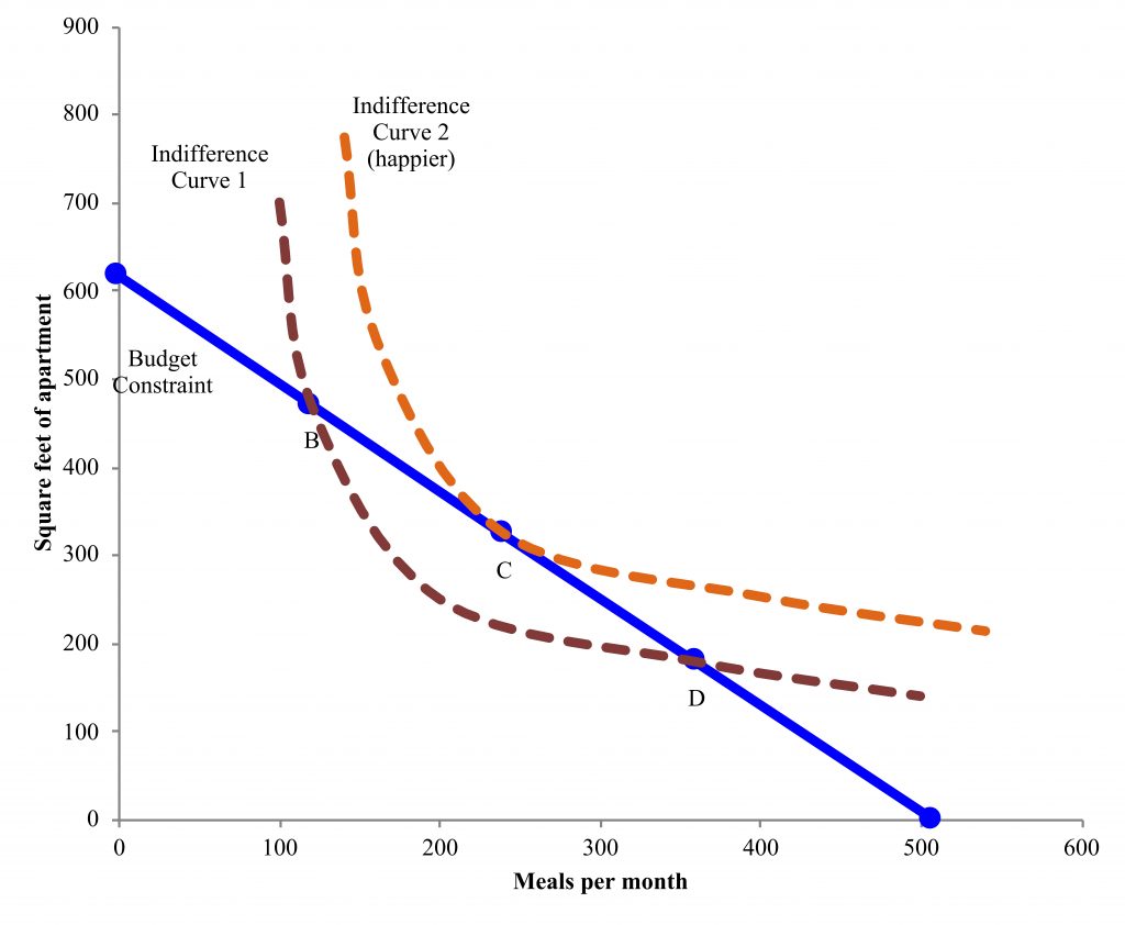
How will this family decide what to do? What trade-offs will they make? To understand the idea of how individuals and families think about tradeoffs, economists use the idea of an indifference curve. An indifference curve shows the combinations of goods that make individuals the same level of “happy,” referred to as utility. So, for instance, the family might be equally happy with only one meal per day but a big apartment (point B) as with 3 meals per day but only renting one bedroom (point D). This combination is shown as indifference curve 1 on Figure 5.3. All the combinations that make a family equally happy are shown on the same indifference curve. Indifference curves that include more of both goods and services (shifted outward) indicate more happiness. People also tend to prefer a mix of goods and services, so point C would be preferred to both B and D (indifference curve 2). People will choose the point that offers them the highest happiness within their budget constraint. In Figure 5.3, this is point C, where indifference curve 2 is just tangent to (touching) the budget constraint.
Production functions: A long run model
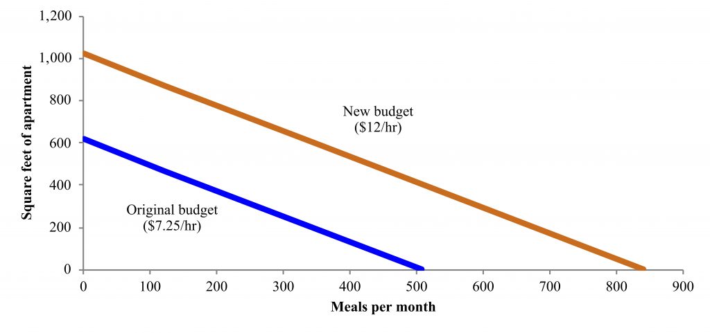
In the long run, it may be possible to shift a family’s budget constraint so they earn more. In order to do this, they would need additional sources of income. Human capital is one potential source of income; because higher-quality human capital (for instance, economic analysis skills) increases productivity, workers will be paid a higher wage (remember that labor demand is determined by workers’ productivity). This increase in productivity is usually modeled with a production function. For instance, a worker may be producing economic analyses, and one input into the production function is their human capital. Raising that human capital increases production (and thus the worker’s productivity). The higher wage will increase (shift out) the worker’s budget constraint. This shift is shown in Figure 5.4, where the family now has their worker earning $12/hour rather than $7.25. Now it is possible for the family to, for example, eat 3 meals a day and have 583 square feet of housing (a studio apartment).
An additional source of income is physical capital, or, when we think about individuals owning physical capital, wealth. Like human capital, physical capital can act as an input into the production function. For instance, a company may buy new sewing machines for their garment factory. If the new sewing machines are faster, this will increase production, since sewing machines are an important element of the garment production function. Individuals may directly own companies, own shares (stocks) in the companies, or own financial capital that is loaned to companies. When they own companies, the physical capital pays off in the long run in higher profits. When individuals own financial capital (stocks), they can receive a financial return, either the payout of a dividend on stocks, or an increase in the cash value of their stocks. When people provide the capital for loans by saving in a bank, they receive a return on their savings (the interest rate they receive). Physical capital can produce a stream of income, which can either be re-invested to generate more, future wealth, in the long run, or can shift out families’ budget constraints. If families who do not have any wealth want to start accruing wealth, they would have to shift their budget constraint inward. They would have to consume less now in order to have a stream of additional income, from their savings becoming wealth and generating a return, in the future.
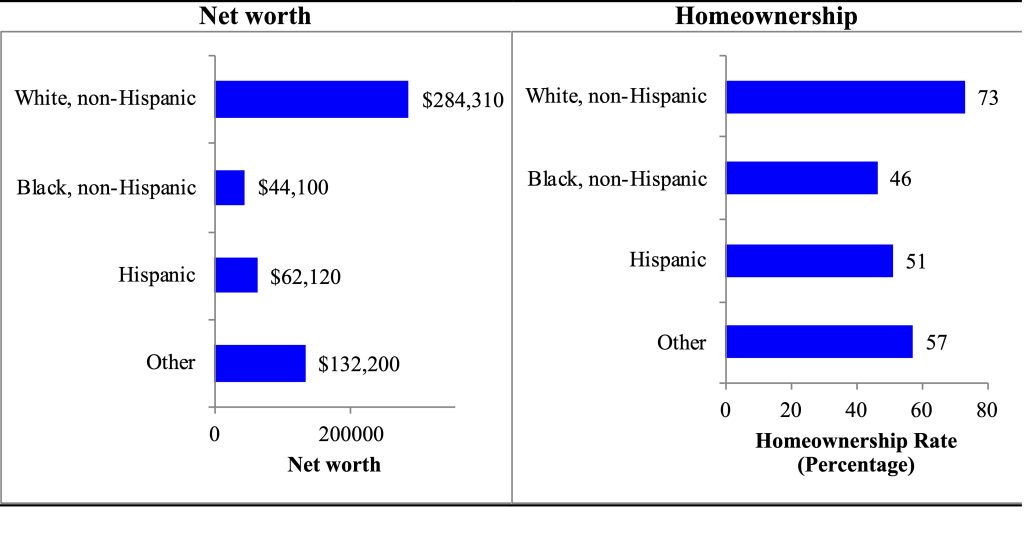
Differences in wealth have an important role in not only current disparities but also perpetuating those disparities across generations. Figure 5.5[10] shows net worth (assets minus liabilities, basically what you own minus what you owe) by race and ethnicity. The figure also shows one of the most common forms of wealth, homeownership. Black, non-Hispanic and Hispanic families have much lower median net worth than white families. Median net worth is $62,120 for Hispanic families and $44,100 for Black, non-Hispanic families compared to $284,310 for White, non-Hispanic families. Differences in homeownership are an important component of wealth disparities, with a 51% rate of homeownership among Hispanic families, 46% among Black, non-Hispanic families, and 73% among White, non-Hispanic families. Historical policies such as redlining (not offering loans in minority communities) as well as ongoing disparities in bank practices contribute to current disparities.[11]
Not only do these disparities in wealth affect income in the present, they also have an intergenerational component, affecting families’ ability to invest in their children. For instance, the low-income family in Figure 5.3 may struggle to feed their children. This food insecurity will reduce the children’s human capital (health and education). Such disparities can be long lasting and affect multiple generations. One of the ways in which slavery in the U.S. continues to affect Black families today is disparities in human capital.[12] Children’s human capital, income, and wealth, are closely linked to that of their parents and even grandparents.[13]
Programs to combat poverty
Programs to combat poverty work to tackle the short run and long run underlying causes of poverty. As well as working on whether families have adequate resources now, programs often aim to shift the underlying human or physical capital of families so that they can move out of poverty. This section looks at a variety of different approaches to combat poverty, including income supports, which expand the budget constraint in the present, as well as investments that can shift budgets in the long run, by increasing human capital or physical capital.
When examining programs to combat poverty in the short run, we are typically thinking about different forms of income supports—to shift families’ budgets outward and allow them to meet more of their basic needs. Income supports come in a variety of forms, including (1) in-kind aid, such as food, (2) conditional cash transfers (cash transfers where recipients have to undertake certain activities or behaviors, such as attending job training or taking children to the doctor) and (3) unconditional cash transfers (receiving cash without any conditions beyond being below a certain income). These different approaches have different impacts on families’ budget constraints as well as their long run human and physical capital.
In-kind aid
Food assistance is a typical type of in-kind aid, targeted to a specific good (food). In the U.S., two important programs that provide assistance with food are the Supplemental Nutrition Assistance Program (SNAP), also known as food stamps, and the Women, Infants, and Children (WIC) program.
Box 5.2: Eligibility and Benefits for SNAP and WIC[14]
Families are typically eligible for SNAP if they (1) are below 130% of the FPL, and (2) have less than $2,500 in resources (bank account balance, cars (in some states), etc.). People have to meet work requirements (working or in a training program) to qualify for SNAP, with some exceptions (children, seniors, pregnant women). Households can receive a maximum allotment that goes down as their income goes up. For each additional dollar of income, a household’s SNAP benefits are reduced by 30 cents. A household of four has a maximum monthly allotment of $835. SNAP benefits are issued on an Electronic Benefit Transfer (EBT) card—like a bank debit card. They can be used for eligible food purchases at participating stores.
WIC provides benefits to women who are pregnant and during the year after a child is born, as well as for infants and children up to five years old. States set income eligibility between 100% and 185% of FPL. Individuals must also be determined to be at nutrition risk. The benefits provided by WIC are vouchers, checks, or EBT to purchase specific nutritious foods such as cereal, fruit/vegetable juice, eggs, milk, cheese, peanut butter, beans/peas, and canned fish. For women with infants who do not breastfeed, WIC provides infant formula.
In-kind food programs shift the budget constraint for only one good. A family with $1,132 in monthly income would receive $309 each month in SNAP benefits. This can only be used for food. We can show this in the budget constraint in Figure 5.6, where the family can buy 127 meals per month with SNAP. This creates the flat section of the budget constraint, where they spend all their cash income on housing (for 566 square feet) and then can choose how much of SNAP to use, up to the maximum SNAP benefit of 127 meals. Past 127 meals, they are facing a similar tradeoff to before; they have to reduce square footage to afford additional meals. However, SNAP still allows for 127 more meals; instead of up to 466 meals per month the family can now afford up to 593.
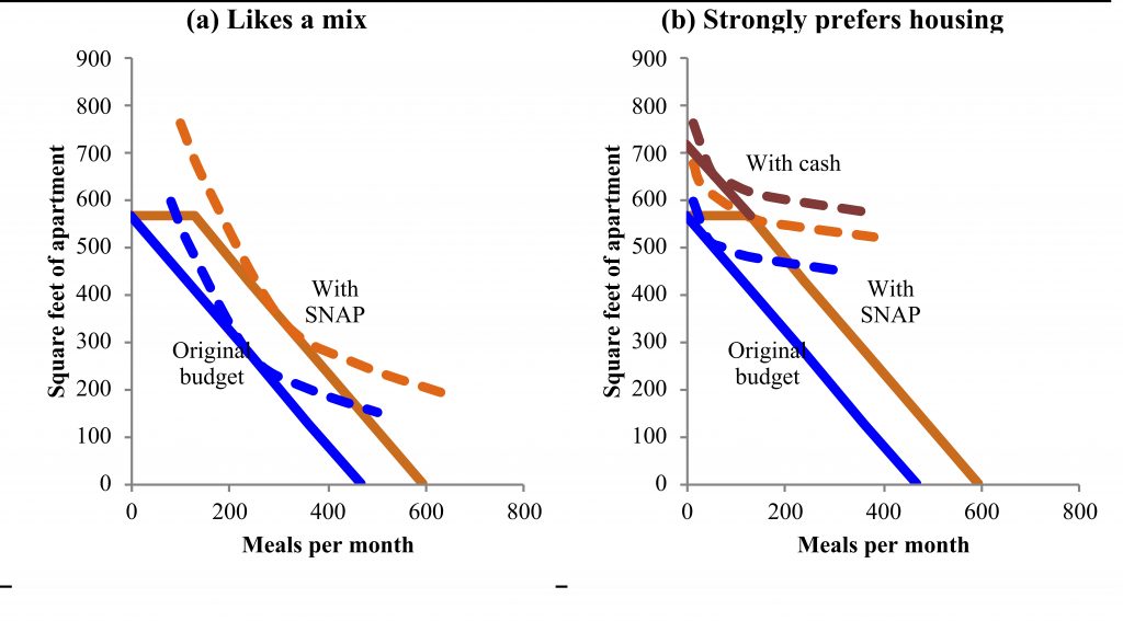
What will the family choose? The answer depends on their preferences (indifference curves). Figure 5.6 shows two possibilities—and an important critique of in-kind income supports. The family in panel (a) likes a mix of both goods; they buy more of both housing and meals with SNAP benefits. They are not restricted by SNAP being only usable for meals because they want to buy more than 127 anyways. This shift in both goods is an example of how benefits are often fungible; for the family in panel (a) SNAP has the same effect as cash would. The family in panel (b) strongly prefers housing. They are restricted by SNAP being only for food; they buy exactly 127 meals with SNAP, but they would actually be happier (on a higher indifference curve) with cash instead. They would buy fewer meals and more housing and be happier. In-kind benefits restrict choice, which will make some families less happy than cash. They also tend to be more administratively burdensome than cash. However, if the goal of the program is to alleviate a particular problem, such as food insecurity, or if there are additional benefits to food consumption (such as accumulation of human capital for children), this may justify the program design.
An additional critique of SNAP and similar income support programs is that they may disincentivize work. If families can meet their basic needs with public benefits, they may choose not to work and instead receive benefits, which is costly to society. SNAP alone would not meet families’ basic needs. However, it may create some work disincentives in how the benefit is determined; for each additional dollar of income families receive 30 cents less in benefits, meaning the net effect of working another hour or getting a raise is only 70% of what it would be without SNAP. We will investigate these sorts of labor disincentives in the next section.
Income support through taxation
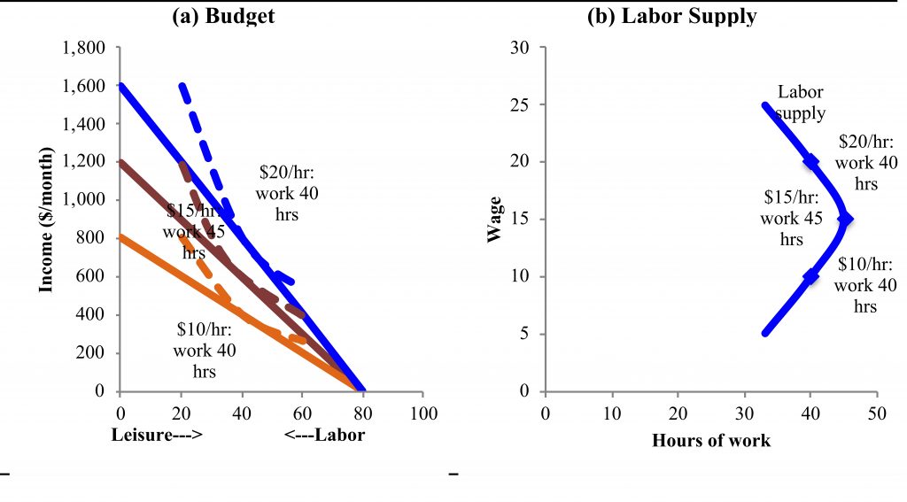
In the U.S. and worldwide, income support is often provided in part through taxation. In this section we will modify our budget constraint model to understand the impact of different tax policies on families’ budgets, and also on their labor supply. In Figure 5.7 we shift our budget constraint to model income and leisure rather than food and housing. It’s important to keep in mind that the opposite of leisure is labor. Assuming that folks have to sleep and care for themselves at least 88 hours a week, the most someone can have work (or leisure) in a week is 80 hours. If they have 80 hours of leisure, they will have an income of zero. For each additional hour that they work, they will have one less hour of leisure, but will have their wage in income (which makes them happy because they will spend that income on their preferred mix of goods and services). The slope of the budget constraint is determined by the wage rate; if the wage is $10, each additional hour of work increases income by $10. Although when the budget constraint increased this usually represented additional amounts of both goods and services, when the wage rate increases, this pivots the budget constraint, because it is only when individuals work another hour that they earn more. Mapping indifference curves, we end up with a backward bending labor supply curve for a worker.
Tax policies can shift the budget constraint. The U.S. and many other countries have progressive tax systems, where individuals with higher incomes pay a higher marginal tax rate. Regressive taxes are taxes where those with lower income pay (relatively) more. The marginal tax rate means that, when an individual moves into a higher tax bracket, he or she does not pay any more taxes on the preceding income, just on additional income. There were seven 2024 tax rates: 10%, 12%, 22%, 24%, 32%, 35%, and 37%. What the brackets encompass in terms of income depends on how someone files, for instance if they are single or married. For a single person earning $15,000 a year, the first $11,600 would be taxed at 10% ($1,160) and the income from $11,600 to $15,000 would be taxed at 12% ($408), for a total tax of $1,568.
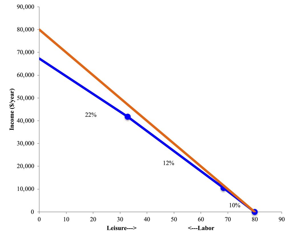
These varying marginal tax rates can be represented in the budget constraint. Figure 5.8 shows, for someone who earns $20 per hour, the different marginal tax rates that shape the budget constraint. As the tax rate increases, the slope of the budget constraint decreases. Although the take-home for each additional hour decreases as the tax rate increases, we know that this is going to have complex effects on labor supply depending on preferences and the shape of our backward bending labor supply curve.
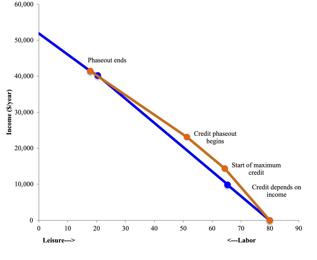
One of the key anti-poverty programs in the U.S., the Earned Income Tax Credit (EITC) uses negative tax rates to try to reduce poverty while incentivizing work. EITC depends on the number of children in the household and filing status. It provides a tax credit (the government pays families) for families depending on their work. The tax credit increases with income up until a maximum point. Figure 5.9 shows the tax credit phasing in for a single mother with one child who makes $15/hour; the credit increases until $12,390 of pre-tax income, when the credit is $4,213. The credit then remains the same amount until $22,720 of pre-tax income. The credit then phases out (goes to zero) by $49,084 of pre-tax income. This shifts out the budget constraint, particularly for the range of 15-30 hours per week, which may not only alleviate poverty but also incentivize work. However, the EITC structure creates an effectively quite high marginal tax rate between $22,720 and $49,084 which may disincentivize work past a certain point. Empirically, EITC has been shown to increase labor supply, especially for single mothers.[15]
Women, who are disproportionately caregivers, face a particular challenge in needing child care for each additional hour they work; the need to pay for child care acts like a tax relative to their budget constraint. Child care will typically be a higher share of their income for women with the lowest incomes, acting like a regressive tax on work. Paying for child care affects both single parents and two-parent households trying to decide whether the second parent should stay at home or work. Child care and other carework costs are a global challenge to economic participation. The loss of women’s domestic labor—child care and other carework along with domestic chores—if they work outside the home plays an important role in low female labor force participation in Egypt. After deducting all their costs, women often find that employment is not worthwhile.[16] In both the U.S. and globally, preschool and kindergarten programs, along with child care subsidies are policies that governments worldwide implement to help alleviate this additional challenge, and also increase the chances of work for women.[17]
Cash aid programs
In the United States, a central program for alleviating poverty for families with children is Temporary Assistance for Needy Families (TANF). This program is what individuals typically mean when they refer to “welfare,” as it provides cash payments to low-income families. The program is for families with children only. TANF, like SNAP and other programs, has both asset and income requirements. Since the program is administered by states, there are different specific policies and benefits in each state. In general, parents are expected to work. TANF provides employment counseling, including training, to aid in finding work. Child care assistance is typically provided with TANF benefits. Benefits are also capped at 60 months (5 years) total for a family. The benefits provided are cash assistance (and coupled with that, SNAP benefits) that depend on the size and income of the family. In Minnesota, the TANF program is called the Minnesota Family Investment Program (MFIP). For a single parent with two children it provides up to $1,394 per month, $16,728 a year in benefits (if the parent does not work).[18] This benefit is not enough to lift families out of poverty; the poverty line for a family of three in 2024 was $25,820.[19]
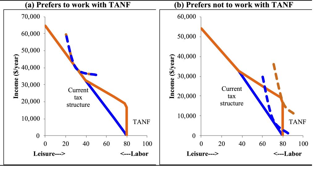
One common concern with programs such as TANF is that they disincentivize work. In some states, beyond a certain (very low) threshold, any additional income reduces the size of the TANF grant dollar-for-dollar. Some states, including Minnesota, phase out the benefits, with families keeping 50 cents of each dollar of additional income up to a certain point. Figure 5.10 shows the budget constraint with TANF where additional income reduces the size of the grant, compared to the current tax structure. In panel (a) the parent prefers to work 50 hours a week at a wage of $18.00 an hour with or without TANF being in place. In panel (b) there is a work disincentive effect; the parent chooses to work 10 hours per week without TANF and no hours with TANF. The parent in (b) is better off (happier, on a higher indifference curve) with TANF than without, but no longer working.
While TANF and welfare have the potential to disincentivize work, there are also work requirements built into the program. These work requirements were part of welfare reform undertaken by President Bill Clinton in 1996.[20] While caseloads (participation) declined after reform, measures of independence, avoiding poverty, and avoiding hardship show less success.[21] The employment effects of reforms are empirically small (for instance, a two percentage point increase in employment by one estimate), but women, especially the poorest women, are financially worse off.[22] Substantial debates remain around the future direction of welfare reform, particularly given that TANF is not effective for families with substantial work barriers, such as temporary disability or domestic abuse.[23]
Box 5.3: Universal Basic Income[24]
One way to alleviate poverty, which is currently being hotly debated around the globe, is to provide a universal basic income (UBI). This is essentially an unconditional guarantee, with no work or any other requirements, of a certain level of income. If the UBI is set above the poverty line, such a policy could instantly alleviate poverty. However, as we have discussed for other anti-poverty programs, UBI could have substantial additional economic effects, including on labor supply. Switzerland recently held a referendum on UBI, as did Finland, The Netherlands, India, and Kenya are all running experiments to study the impact of UBI. One experiment that was undertaken in the 1970s in Manitoba suggests that, while UBI did reduce women’s labor supply, it also improved health. Additional, more recent experiments will be helpful in understanding the impact of UBI in different contexts.
Human Capital Investments
In the long run, poverty alleviation requires shifting families’ human or physical capital to increase their productivity and income. This section discusses some of the evidence on human capital investments as a poverty alleviation strategy. One common global policy that combines elements of cash aid and human capital investment is a conditional cash transfer (CCT). CCTs use means tests, assessing a families’ assets to identify families in poverty or otherwise at risk for poor human capital accumulation. Means tests are used because cash income is often a difficult measure to implement in developing countries. CCTs provide cash aid conditional on families’ behavior; in developing countries where health, malnutrition, and school drop outs are common problems, CCTs often condition on families’ taking children for medical visits, nutrition evaluations, or school enrollment. The conditionality is in part because families might not make these investments otherwise, because such investments may not pay off to the parents, but rather to their children, or because there are market failures preventing them from making such investments. CCTs improve education and nutrition outcomes, usually (but not always) to a greater extent than unconditional programs.[25] CCTs also tend to provide transfers to women, because they usually (but not always) will invest more in the next generation.[26]
A variety of poverty alleviation programs target the human capital of children at risk of poverty directly, instead of through conditions. Nurse visitation programs, which provide prenatal and infancy home visits to promote maternal and child health and development, improve various aspects of both parents’ and children’s development, including reducing the use of other poverty alleviation programs.[27] High quality early childhood programs improve education and earnings outcomes, decreasing use of welfare and other social assistance programs.[28] School meal (breakfast and lunch) programs have both short-term nutrition effects and long-run educational effects.[29] All of these are effective programs for improving human capital early in life.
For adults, alleviating poverty through human capital interventions is more challenging, in part because much of human capital is shaped during the early years of life. Training programs, which can confer additional human capital, tend to be ineffective in the short term, but may have medium term impacts.[30] Currently there are a large number of job training programs in the U.S. targeting the unemployed and low-income workers. For training programs to be effective, they need to confer the skills in demand in the labor market, which can be challenging for public programs and requires substantial information about the skills employers seek.[31]
Physical Capital: Wealth and Neighborhoods
In order for families to acquire wealth, and from that a stream of income, they must be able to save. Programs to increase saving have particularly targeted low-income countries, where microcredit programs provide small loans, typically to start a business, and often targeted to women who face particular barriers to finance. Microsavings programs, including group savings, may also help low-income families accumulate capital. The balance of evidence is that microfinance programs have at most modest positive effects on households.[32] Microsavings programs, with savings products designed or subsidized for low-income families, do have large savings and wealth impacts.[33]
Neighborhoods can play a role in poverty; whether a family lives in an area with a high concentration of poverty can affect their outcomes, in part through the services they can access and in part due to their social networks (social capital). Moving families to areas with less concentrated poverty has been suggested as one intervention that can help reduce poverty. Moving families can improve outcomes in some contexts, with positive impacts observed in the U.S.[34] A program that randomly relocated families in India from slums to improved housing on the edge of the city did not have positive long-term outcomes, in part due to the fact that it disconnected families from their social networks.[35]
Conclusions
What can we do to alleviate poverty for families around the world? In the short run, we can shift out families’ budget constraints by providing them with more resources. In-kind aid, such as food stamps, can improve their well-being, but often has the same effect as cash. Income supports that provide cash have potential work disincentive effects, but programs such as the EITC can actually incentivize work through tax credits. In either case, with both TANF (welfare) and EITC, the labor supply effects of programs tend to be relatively small.
In the long-run, increasing human capital, through investments in children’s health or adults’ skills, plays an important role in increasing individuals’ productivity, ultimately alleviating poverty. Likewise, increases in wealth (physical capital), through savings or loans, as well as geographic mobility can play an important role in long-run poverty alleviation. Although there has been substantial progress in reducing global poverty, in the U.S. poverty has been a persistent problem for adults and children for decades. The elderly have, however, through Social Security, experienced major decreases in poverty since the 1960s. Identifying programs, such as basic incomes, that can achieve similar results for children and families is an important agenda for economic research in the near future.
List of terms
- Federal poverty line (FPL)
- Budget constraint
- Production function
- In-kind aid
- Conditional cash transfers
- Unconditional cash transfers
- Supplemental Nutrition Assistance Program (SNAP)
- Women, Infants, and Children Program (WIC)
- Indifference curve
- Progressive taxes
- Regressive taxes
- Earned Income Tax Credit (EITC)
- Temporary Assistance for Needy Families (TANF)
- Microcredit
- Microsavings
References
Almeida, Rita, Jere Behrman, and David Robalino. 2012. The Right Skills for the Job? Rethinking Training Policies for Workers. Human Development Perspectives. Washington, DC: World Bank.
Angelucci, Manuela, Dean Karlan, and Jonathan Zinman. 2015. “Microcredit Impacts: Evidence from a Randomized Microcredit Program Placement Experiment by Compartamos Banco.” American Economic Journal: Applied Economics 7 (1): 151–182.
Augsburg, Britta, Ralph De Haas, Heike Harmgart, and Costas Meghir. 2015. “The Impacts of Microcredit: Evidence from Bosnia and Herzegovina.” American Economic Journal: Applied Economics 7 (1): 183–203.
Baird, Sarah, Craig McIntosh, and Berk Ozler. 2011. “Cash or Condition? Evidence from a Cash Transfer Experiment.” The Quarterly Journal of Economics 126 (4): 1709–1753.
Banerjee, Abhijit, Esther Duflo, Rachel Glennester, and Cynthia Kinnan. 2015. “The Miracle of Microfinance? Evidence from a Randomized Evaluation.” American Economic Journal: Applied Economics 7 (1): 22–53.
Barnhardt, Sharon, Erica Field, and Rohini Pande. 2017. “Moving to Opportunity or Isolation? Network Effects of a Randomized Housing Lottery in Urban India.” American Economic Journal: Applied Economics 9 (1): 1–32.
Bassett, Lucy. 2008. “Can Conditional Cash Transfer Programs Play a Greater Role in Reducing Child Undernutrition?” World Bank Social Protection Discussion Paper Series No. 835. Washington DC.
BBC News. 2016. “Switzerland’s Voters Reject Basic Income Plan.” BBC News (June 5).
Benhassine, Najy, Florencia Devoto, Esther Duflo, Pascaline Dupas, and Victor Pouliquen. 2015. “Turning a Shove into a Nudge? A ‘Labeled Cash Transfer’ for Education.” American Economic Journal: Economic Policy 7 (3): 1–48.
Bertocchi, Graziella. 2016. “The Legacies of Slavery in and out of Africa.” IZA Journal of Migration 5 (4). IZA Journal of Migration: 1–19.
Bhattacharya, Jayanta, Janet Currie, and Steven J. Haider. 2006. “Breakfast of Champions? The School Breakfast Program and the Nutrition of Children.” Journal of Human Resources 41 (3): 445–466.
Blank, Rebecca M., and Mark H. Greenberg. 2008. “Improving Measurement of Poverty.” The Hamilton Project Discussion Paper No. 2008–17.
Cancian, Maria, and Daniel R. Meyer. 2004. “Alternative Measures of Economic Success among TANF Participants: Avoiding Poverty, Hardship, and Dependence on Public Assistance.” Journal of Policy Analysis and Management 23 (3): 531–548.
Card, David, Jochen Kluve, and Andrea Weber. 2010. “Active Labour Market Policy Evaluations: A Meta‐Analysis.” The Economic Journal 120: 452–477.
Connelly, Rachel. 1992. “The Effect of Child Care Costs on Married Women’s Labor Force Participation.” The Review of Economics and Statistics 74 (1): 83–90.
Crépon, Bruno, Florencia Devoto, Esther Duflo, and William Pariente. 2015. “Estimating the Impact of Microcredit on Those Who Take It Up: Evidence from a Randomized Experiment in Morocco.” American Economic Journal: Applied Economics 7 (1): 123–150.
Danziger, Sandra K., Sheldon Danziger, Kristin S. Seefeldt, and H. Luke Shaefer. 2016a. “From Welfare to a Work-Based Safety Net: An Incomplete Transition.” Journal of Policy Analysis and Management 35 (1): 231–238.
———. 2016b. “Increasing Work Opportunities and Reducing Poverty Two Decades After Welfare Reform.” Journal of Policy Analysis and Management 35 (1): 241–244.
Duflo, Esther. 2003. “Grandmothers and Granddaughters: Old Age Pension and Intra-Household Allocation in South Africa.” World Bank Economic Review 17 (1): 37.
Eckenrode, John, Mary Campa, Dennis W. Luckey, Charles R. Henderson, Robert Cole, Harriet Kitzman, Elizabeth Anson, Kimberly Sidora-Arcoleo, Jane Powers, and David Olds. 2010. “Long-Term Effects of Prenatal and Infancy Nurse Home Visitation on the Life Course of Youths: 19-Year Follow-up of a Randomized Trial.” Archives of Pediatrics & Adolescent Medicine 164 (1): 9–15.
Eissa, Nada, and Jeffrey B Liebman. 1996. Labor Supply Response to the Earned Income Tax Credit. NBER Working Paper Series. Vol. 111.
England, Charlotte. 2017. “Indian Government Survey Says Universal Basic Income Could Combat Poverty.” The Independent Online (January 31).
Federal Reserve. 2023. “The Fed – Table – Survey of Consumer Finances, 1989- 2022.” Survey of Consumer Finances.
Fisher, Gordon M. 2008. “Mollie Orshansky: Author of the Poverty Thresholds.” Amstat News, September.
Fiszbein, Ariel, Norbert Schady, Francisco H. G. Ferreira, Margaret Grosh, Nial Kelleher, Pedro Olinto, and Emmanuel Skoufias. 2009. Conditional Cash Transfers: Reducing Present and Future Poverty. Washington, DC: World Bank.
Fitzpatrick, Maria Donovan. 2010. “Preschoolers Enrolled and Mothers at Work? The Effects of Universal Prekindergarten.” Journal of Labor Economics 28 (1): 51–85.
Fitzpatrick, Maria Donovan. 2012. “Revising Our Thinking About the Relationship Between Maternal Labor Supply and Preschool.” Journal of Human Resources 47 (3): 583–612.
Forget, Evelyn L. 2011. “The Town with No Poverty: The Health Effects of a Canadian Guaranteed Annual Income Field Experiment.” Canadian Public Policy 37 (3): 283–305.
Gertler, Paul. 2004. “Do Conditional Cash Transfers Improve Child Health? Evidence from PROGRESA’s Control Randomized Experiment.” The American Economic Review 94 (2): 336–341.
Gitter, Seth R., and Bradford L. Barham. 2008. “Women’s Power, Conditional Cash Transfers, and Schooling in Nicaragua.” World Bank Economic Review 22 (2): 271–290.
Hanna, Rema, and Benjamin A. Olken. 2018. “Universal Basic Incomes versus Targeted Transfers: Anti-Poverty Programs in Developing Countries.” Journal of Economic Perspectives 32 (4): 201–226.
Hinrichs, Peter. 2010. “The Effects of the National School Lunch Program on Education and Health.” Journal of Policy Analysis and Management 29 (3): 479–505.
Hoodfar, Homa. 1997. Between Marriage and the Market: Intimate Politics and Survival in Cairo. Berkeley, CA: University of California Press.
Hoynes, Hilary W., Marianne E. Page, and Ann Huff Stevens. 2006. “Trends and Explanations.” Journal of Economic Perspectives 20 (1): 47–68.
Karlan, Dean, Aishwarya Lakshmi Ratan, and Jonathan Zinman. 2014. “Savings by and for the Poor: A Research Review and Agenda.” Review of Income and Wealth 60 (1): 36–78.
Kimmel, Jean. 1998. “Child Care Costs as a Barrier to Employment for Single and Married Mothers.” Review of Economics and Statistics 80 (2): 287–299.
Kling, Jeffrey R., Jens Ludwig, and Lawrence F. Katz. 2013. “Neighborhood Effects on Crime for Female and Male Youth: Evidence from a Randomized Housing Voucher Experiment.” Quarterly Journal of Economics 120 (1): 87–130.
Lang, Kevin. 2007. Poverty and Discrimination. Princeton, NJ: Princeton University Press.
Lowrey, Annie. 2017. “The Future of Not Working.” The New York Times (February 23).
Ludwig, Jens, Greg J. Duncan, and Paul Hirschfield. 2001. “Urban Poverty and Juvenile Crime: Evidence from a Randomized Housing-Mobility Experiment.” The Quarterly Journal of Economics 116 (2): 655–679.
Meyer, Bruce D., and Dan T. Rosenbaum. 2001. “Welfare, the Earned Income Tax Credit, and the Labor Supply of Single Mothers.” The Quarterly Journal of Economics 116 (3): 1063–1114.
Meyers, Marcia K., Theresa Heintze, and Douglas A. Wolf. 2002. “Child Care Subsidies and the Employment of Welfare Recipients.” Demography 39 (1): 165–79.
Minnesota Department of Human Services. 2024. “MFIP/DWP Assistance Standards.” Retrieved October 2, 2024. https://www.dhs.state.mn.us/main/idcplg?IdcService=GET_DYNAMIC_CONVERSION&dDocName=cm_002009&RevisionSelectionMethod=LatestReleased.
Olds, David L. 2007. “Preventing Crime with Prenatal and Infancy Support of Parents: The Nurse-Family Partnership.” Victims & Offenders 2: 205–225.
Olds, David L., Harriet Kitzman, Robert Cole, JoAnn Robinson, Kimberly Sidora, Dennis W. Luckey, Charles R. Henderson, Carole Hanks, Jessica Bondy, and John Holmberg. 2004. “Effects of Nurse Home-Visiting on Maternal Life Course and Child Development: Age 6 Follow-up Results of a Randomized Trial.” Pediatrics 114 (6): 1550–9.
Orshansky, Mollie. 1965. “Counting the Poor: Another Look at the Poverty Profile.” Social Security Bulletin.
Prescott, David, Robert Swidinsky, and David A. Wilton. 1986. “Labour Supply Estimates for Low-Income Female Heads of Household Using Mincome Data.” The Canadian Journal of Economics 19 (1): 134–141.
Sacerdote, Bruce. 2005. “Slavery and the Intergenerational Transmission of Human Capital.” The Review of Economics and Statistics 87 (2): 217–234.
Schreck, Niccole. 2016. “Rental Reality: What You Can Expect to Pay in 10 Major U.S. Cities.” U.S. News & World Report (January 4).
Social Security Administration. 2016. “Fact Sheet: Social Security.”
Sullivan, Laura, Tatjana Meschede, Lars Dietrich, Thomas Shapiro, Amy Traub, Catherine Ruetschlin, and Tamara Draut. 2015. “The Racial Wealth Gap: Why Policy Matters.” Demos & IASP.
Tanner, Michael. 1996. The End of Welfare: Fighting Poverty in the Civil Society. Washington, DC: Cato Institute.
Tarozzi, Alessandro, Jaikishan Desai, and Kristin Johnson. 2015. “The Impacts of Microcredit: Evidence from Ethiopia.” American Economic Journal: Applied Economics 7 (1): 54–89.
Temple, Judy A., and Arthur J. Reynolds. 2007. “Benefits and Costs of Investments in Preschool Education: Evidence from the Child–Parent Centers and Related Programs.” Economics of Education Review 26 (1): 126–144.
U.S. Census Bureau. 2024. “Data: Historical Poverty Tables: People and Families – 1959 to 2023.” Retrieved October 2, 2024. https://www.census.gov/data/tables/time-series/demo/income-poverty/historical-poverty-people.html.
U.S. Department of Health & Human Services–Office of the Assistant Secretary for Planning and Evaluation. 2024. “Poverty Guidelines.” Retrieved October 2, 2024. https://aspe.hhs.gov/poverty-guidelines.
USDA. 2016. “Women, Infants and Children (WIC) Frequently Asked Questions.” Retrieved February 26, 2017. https://www.fns.usda.gov/wic/frequently-asked-questions-about-wic#5.
———. 2017a. “Official USDA Food Plans: Cost of Food at Home at Four Levels, U.S. Average, January 2017.”
———. 2017b. “Women, Infants and Children (WIC): Eligibility Requirements.” Retrieved February 26, 2017. https://www.fns.usda.gov/wic/wic-eligibility-requirements.
———. 2021. “Supplemental Nutrition Assistance Program (SNAP): Eligibility.” Retrieved August 29, 2021. https://www.fns.usda.gov/snap/eligibility.
World Bank. 2007. “Arab Republic of Egypt Poverty Assessment Update.” Washington, DC: World Bank.
Ziliak, James P. 2015. “Temporary Assistance for Needy Families.” National Bureau of Economic Research Working Paper Series No. 21038.
- U.S. Department of Health & Human Services--Office of the Assistant Secretary for Planning and Evaluation 2024 ↵
- World Bank 2007 ↵
- Blank and Greenberg 2008; Tanner 1996 ↵
- Fisher 2008; Orshansky 1965 ↵
- U.S. Census Bureau 2024 ↵
- Social Security Administration 2016 ↵
- Hoynes, Page, and Stevens 2006 ↵
- USDA 2017a ↵
- Schreck 2016 ↵
- Federal Reserve 2023 ↵
- Sullivan et al. 2015 ↵
- Bertocchi 2016 ↵
- Sacerdote 2005 ↵
- USDA 2017b; 2016; 2021 ↵
- Eissa and Liebman 1996; Meyer and Rosenbaum 2001 ↵
- Hoodfar 1997 ↵
- Connelly 1992; Fitzpatrick 2010; 2012; Kimmel 1998; Meyers, Heintze, and Wolf 2002 ↵
- Minnesota Department of Human Services 2024 ↵
- U.S. Department of Health & Human Services--Office of the Assistant Secretary for Planning and Evaluation 2024 ↵
- Danziger et al. 2016a ↵
- Cancian and Meyer 2004 ↵
- Ziliak 2015 ↵
- Danziger et al. 2016b ↵
- BBC News 2016; England 2017; Forget 2011; Hanna and Olken 2018; Lowrey 2017; Prescott, Swidinsky, and Wilton 1986 ↵
- Baird, McIntosh, and Ozler 2011; Benhassine et al. 2015 ↵
- Benhassine et al. 2015; Duflo 2003; Gitter and Barham 2008 ↵
- Eckenrode et al. 2010; Olds 2007; Olds et al. 2004 ↵
- Temple and Reynolds 2007 ↵
- Bhattacharya, Currie, and Haider 2006; Hinrichs 2010 ↵
- Card, Kluve, and Weber 2010 ↵
- Almeida, Behrman, and Robalino 2012 ↵
- Angelucci, Karlan, and Zinman 2015; Augsburg et al. 2015; Banerjee et al. 2015; Crépon et al. 2015; Tarozzi, Desai, and Johnson 2015 ↵
- Karlan, Ratan, and Zinman 2014 ↵
- Kling, Ludwig, and Katz 2013; Ludwig, Duncan, and Hirschfield 2001 ↵
- Barnhardt, Field, and Pande 2017 ↵
