Lab #8 One-Way ANOVA

In this laboratory you will learn how to:

• Load an SPSS data file
• Compute and interpret a one-way ANOVA
• Compute and interpret ANOVA post-hoc tests

Introduction

Many research scenarios require comparison of more than two samples or conditions. While it may be possible to compute multiple t-tests, this approach has a variety of problems and becomes increasingly unwieldy as the number of samples or conditions increases. These problems are alleviated through a statistical method called Analysis of Variance (ANOVA). In ANOVA, an F-test is used to determine whether any differences exist among the groups or conditions. If there are differences, post-hoc testing is done to locate the groups or conditions that differ significantly from one another. As noted in the “Lab Preview” document, ANOVA hypotheses are always non-directional; we are testing the null of no differences between means.

For this laboratory, we will again be using the SPSS data file called “hourlywagedata.sav”. We used this data file in a previous lab so you should already have a copy on your computer. If you are unable to locate the file, you can download it from the SPSS Data Files section of this book or from our course area in D2L Brightspace.

As you may recall, these data are from a sample of 3000 nurses. Several pieces of information were collected for each nurse including type of nurse (position), age category (agerange), years of experience category (yrsscale), and hourly salary (hourwage). As you observed in the previous lab, there are three age categories (18-30, 31-45, or 46-65) and six years of experience categories (5 or less, 6-10, 11-15, 16-20, 21-35, or 36+).

In this laboratory we will be using ANOVA to compare hourly salaries for nurses across the three different age categories and across the six levels of experience categories. Thus, we will be using agerange and yrsscale as our independent variables (technically quasi-IVs because they are not manipulated; the terminology for an IV in ANOVA is a “factor”) and hourwage is our dependent (outcome) variable.

Start SPSS and Load the Data

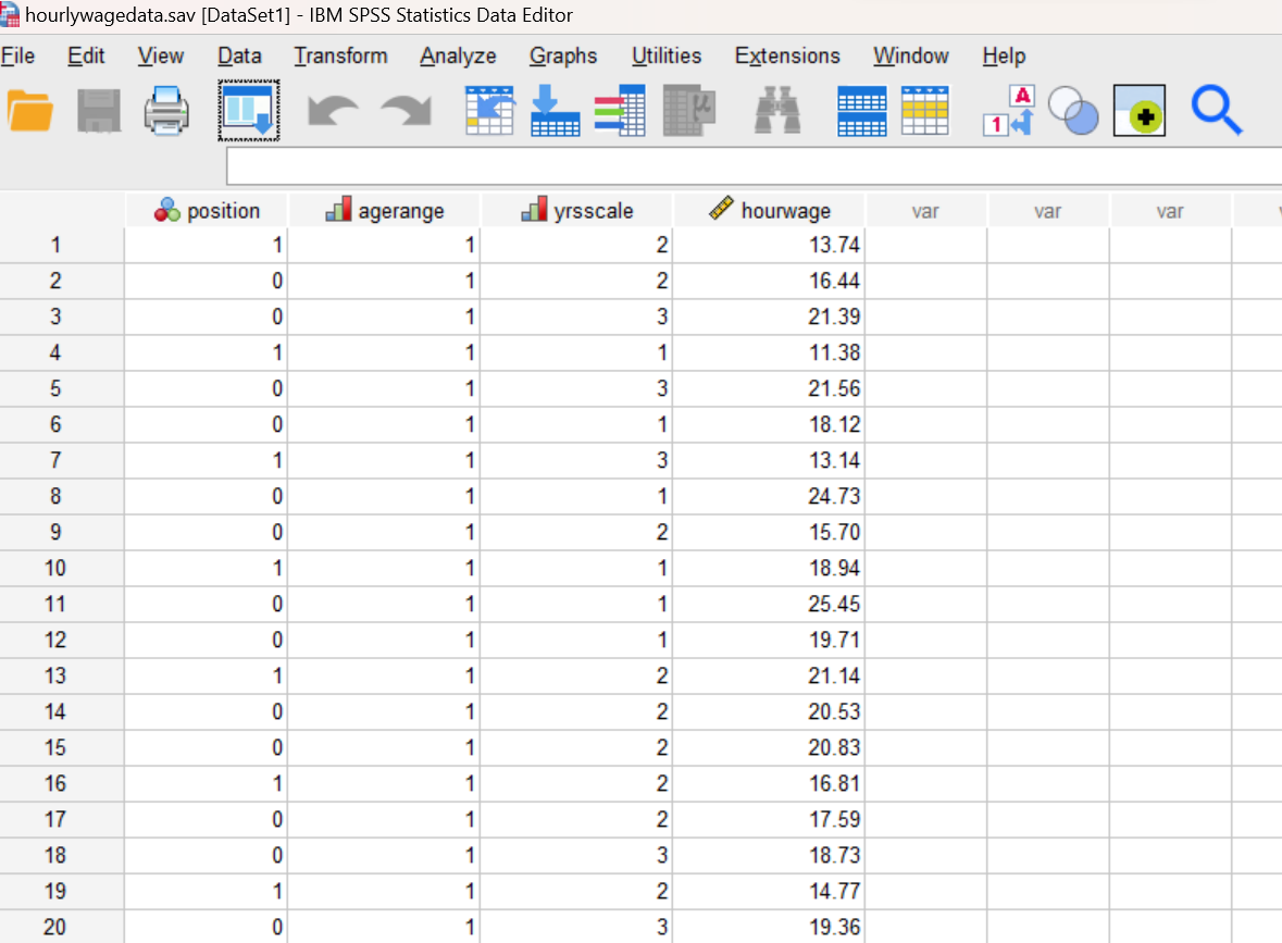
Start SPSS as you have done in previous labs, using your application menu or program search tool and load the “hourlywagedata.sav” data file into your Data Editor. At this point, your Data Editor window should be displaying the data as shown here:

Compute Descriptive Statistics

It is always a good idea to start your analysis using descriptive statistics. This approach allows you to look for unusual patterns (possibly miscoded data) and violations of assumptions of any statistical tests you are planning to run. For this lab, though, we are going to shorten this step since we have used this dataset before and you should be very familiar with running various descriptive statistics commands by now. Thus, we aren’t going to get the means in table form, but instead create a graph to see the means – and how they compare across groups – in a visual form.

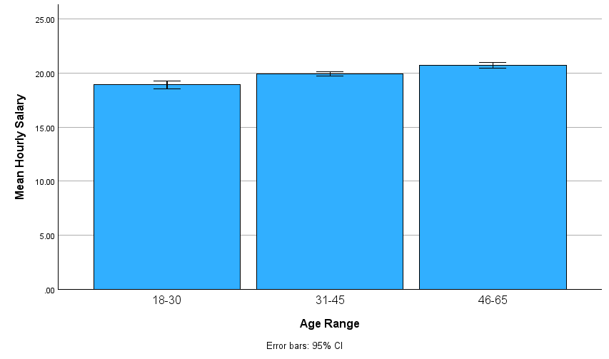
Use the SPSS menu system to create a bar chart (Graphs→Bar) showing how hourly salary (hourwage) varies across the three age categories (agerange), with 95% confidence intervals shown for each mean. You learned how to create this type of chart in Lab #4, so refer back to those instructions if you need to refresh your memory on how to set things up. Remember that you need to click on “Other statistic” and request that the mean be used for each bar, and also go into the Options menu to request the 95% CI error bars. Once you have set up and generated the chart correctly, it should look similar to the following:

Annotate Your Examine Output

Insert some text into your Statistics Viewer window at this point to describe the graph you have just produced and give your interpretation of the results. How do the means compare across the three categories; do older nurses earn higher salaries as one might expect? Are any differences still relevant when considering the margin of error (95% CIs) as shown on the graph? Remember to write out your interpretation in complete sentences.

One-way Analysis of Variance (ANOVA)

Now that we have a good general understanding of the data we will be working with, let’s use one-way analysis of variance to statistically compare the mean hourly salary across the three age categories. The first step in making comparisons among the means is to test the null hypothesis that all of the means are the same. Note that this test will not tell you where any differences are located (that is, which groups are different), only whether there are some differences among the means.

In SPSS, the ONEWAY command is used for analysis of variance as long as there is only one independent variable. (Multiple dependent variables can be specified, in which case SPSS will compute a one-way ANOVA for each dependent variable, but we will not be doing that in this lab.) Open a new Syntax Editor window (File→New→Syntax) and type the following command:

Run the command and examine the output in your Statistics Viewer window. It should look similar to what is shown below. You should notice that this command produces four tables. The first table shows descriptive statistics for the groups being compared, the second table shows the results of Levene’s test for homogeneity of variances, the third table shows the results of the hypothesis test in the format of a standard ANOVA summary table, and the fourth table shows the effect size for the F-test.

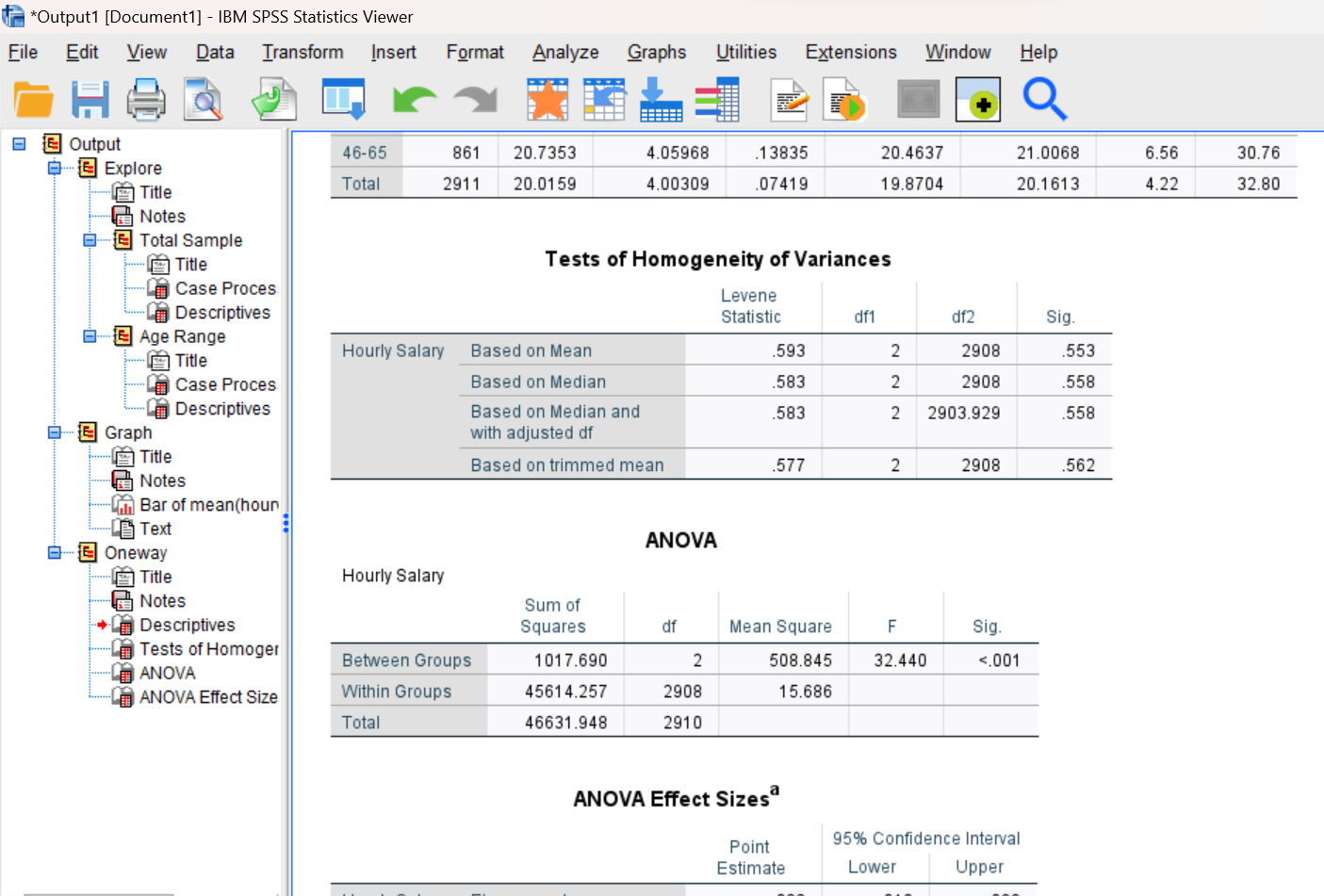
As for the independent samples t-test (Lab #6), we will first want to check that the variances of the groups do not differ significantly, using Levene’s test. SPSS actually reports several versions of Levene’s test in this table. We will use the one in the top row (Based on Mean). Remember that if Levene’s test produces a significance (Sig.) value greater than your alpha level (use alpha = .05), you can consider the homogeneity of variances assumption to be satisfied.

Interpreting the ANOVA F-test

In looking at the ANOVA summary table, you will find information on the sum of squares, df, and mean square for both between and within group variance, which are used to calculate the F statistic. As a reminder, the degrees of freedom (which you will need to indicate below) is the number of group means minus one (k – 1) for df between (the numerator for the F) and the number of total people in the study minus the number of groups for df within (N – k; or  n₁-1 + n₂-1 + n₃-1 + etc. for the number of groups; the denominator for the F).

Your goal in interpreting this ANOVA table is to determine whether you can reject the null hypothesis. If the reported significance (Sig.) value here is less than your alpha level (use alpha = .05), you can reject the null hypothesis and conclude there is/are some significant difference(s) in hourly salaries among the group means. If the significance value is greater than your alpha level, you will fail to reject the null hypothesis and conclude there are no statistical differences among the group means.

Interpreting Effect Size

Note that SPSS produces a measure of effect size called eta-squared (ƞ2) for the ANOVA F-test. SPSS displays a few variations of this effect size measure, but for the purposes of this class, we will just use the one in the top row of the table (the one labeled Eta-squared). Eta-squared measures the proportion of variance accounted for by the independent variable (factor). Guidelines for interpreting this measure of effect size are as follows:

Annotate Your ANOVA F-Test Results

Add some text into your output to interpret your results from the ANOVA F-test. Report the information IN THIS ORDER, and separated by letter so each piece is clearly identified! (We will skip the APA style result statement for now but will add it later after we run our next analysis.)

1. Report the results of Levene’s test. You should include a report of the p value (Sig.) and a statement indicating whether the assumption of homogeneity of variances has been satisfied and how you determined that.
2. Report the sample means being compared in this analysis. Report the F, df (remember, there are two of them!), and p value (Sig.) for the test; use the APA style F-statement if you want to, or just list things out.
3. State your statistical decision about the null hypothesis – which, as always, is either to reject or fail to reject – and state why you made that decision. Does your decision about the null hypothesis indicate that there are or are not differences between the mean hourly salaries across the age groups?
4. Report your eta-squared value (which you can find in the fourth table) and include an interpretation of the size of the effect using the guidelines given above.

Compute Post-Hoc Pairwise Comparisons

A non-significant F test in the one-way ANOVA tells you there are no significant differences among the groups. A significant F test, on the other hand, tells you there is at least one significant difference among the groups, but it does not tell you exactly which group means differ significantly. Further testing is necessary to determine where the differences are located. This can be accomplished using post-hoc tests. SPSS provides a wide variety of post-hoc tests including the commonly used Tukey and Scheffé tests. We will make use of the Tukey test here.

Return to your Syntax Editor and use the following command to determine which age groups differ significantly from one another in their hourly salaries.

After running the command, review the output in your Statistics Viewer window. You will want to focus on the Multiple Comparisons table, which should look similar to the following:

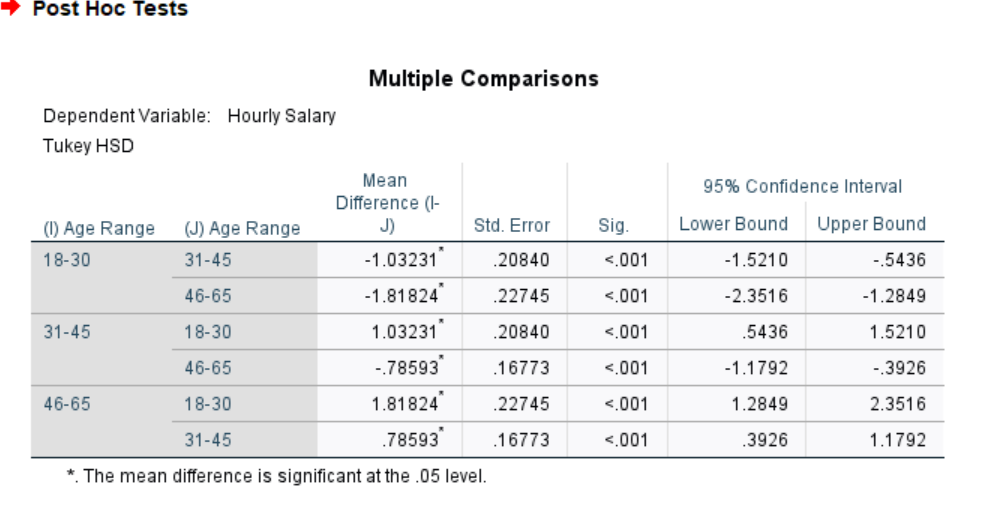
For each pair of age ranges, SPSS displays the difference between the two means and a p value (labeled as Sig. in the table) for the pairwise comparison. As usual, if the p value is less than your alpha level (.05), you can conclude the difference between those two means is statistically significant. An asterisk (*) beside the mean difference also serves as an indicator that the difference is statistically significant at the alpha level you have specified.

Annotate Your Post-Hoc Test Results

First, summarize the results of the Tukey post-hoc test: which means are significantly different from one another? You could do this by listing out each pair of means and noting if the two means are or are not different (e.g., is age 18-30 different or not from age 31-45? Is age 18-30 different or not from age 46-65? And is age 31-45 different or not from age 46-65?), or possibly find a way to summarize the results in a more concise way.

Second, write a paragraph summarizing the “real world” results for this analysis. Try to write things out in APA style. Check the Lab Preview document for examples and information about how to write the F-statement (like what to include for degrees of freedom). As with those examples, start with an overall statement about whether there was or was not a difference between the means for your variables according to the ANOVA, with the F-statement at the end. Then, write a sentence or two that reports the three group means (with standard deviations) and explain how/where the significant differences between means were based on the post-hoc tests, making sure to identify higher/lower/same hourly wages for each pair.

ANOVA for hourwage by Years of Experience

Now, let’s repeat these same analyses using the SPSS menu system, but this time with years of experience category (yrsscale) as the factor (independent variable) and hourwage again as our dependent variable.

We’ll skip the descriptive statistics step again (we’ll get them when we run the ANOVA), but start by creating a bar chart (Graphs→Bar) showing how hourly salary (hourwage) varies for nurses in the six different experience categories (yrsscale). The bars in your chart should represent the mean of the hourwage variable for each of the yrsscale categories. Set up your bar chart as you did earlier in the lab. Again, remember to select “Other statistic” and request the mean to be displayed for each bar and add the 95% CI error bars. After generating your bar chart, it should look like what is shown here:

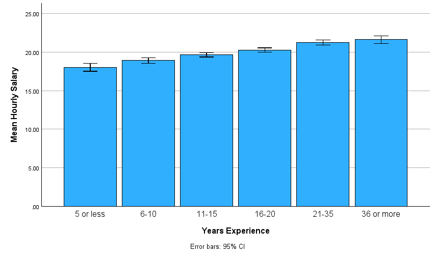
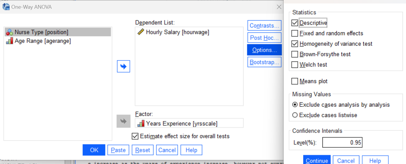
Now let’s run the actual ANOVA for comparing the mean hourly salaries for these six groups of nurses. Using the menu system, you can find the oneway analysis of variance in the Analyze menu under Compare Means and Proportions (Analyze→Compare Means and Proportions→One-Way ANOVA). Navigate to this command now, and in the resulting dialog box, move your hourwage variable to the Dependent list and your yrsscale variable to the Factor box as shown below (as mentioned earlier, “factor” is the term for the IV/grouping variable in ANOVA). Be sure to check the box to Estimate the effect size. Also, unlike t-tests, we do need to change the options here: Click on the Options button and check the boxes for Descriptive statistics and Homogeneity of variance test or you will not get those tables in your output!

Press the OK button to run the command and review your results in the Statistics Viewer window. Is the homogeneity of variances assumption satisfied? Are there differences in hourly salaries among these six experience levels? Look at your ANOVA table; is the p value less than .05?

To determine exactly which means differ from one another, you will need to run a post-hoc test. We’ll use the Tukey test again here. Navigate back in the menu system to your previous ANOVA command (Analyze→Compare Means and Proportions→One-Way ANOVA) and in the resulting dialog box, click on the Post Hoc button. This will take you to a list of all the post hoc testing options that are available in SPSS as shown here:

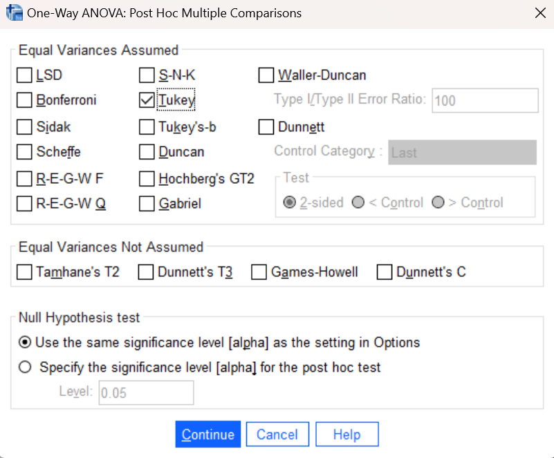
Select the check box for Tukey and press the Continue button. You can also go into the Options menu and un-select what we asked for before (Descriptives and Homogeneity of variances test); if you don’t, you’ll just get those same results again and can delete the duplicate tables. Press the OK button in the original dialog box and your previous ANOVA will be run again, but this time with a Multiple Comparisons table for the Tukey test (it will be quite a bit larger this time since we are comparing six groups!). Examine your results in the Statistics Viewer and locate the significant mean differences.

Annotate Your ANOVA and Post-Hoc Results

Insert the following into your output to interpret your results from the ANOVA F-test. Report the information IN THIS ORDER, and separated by letter so each piece is clearly identified! A full APA style statement is not required for this analysis (see notes below), although you are free to write in APA Style as much as you wish to since that provides a guide for how to discuss results!

1. Report the results of Levene’s test for Homogeneity of Variances. Was this assumption satisfied?
2. Report the sample means being compared in this analysis. Report F, df (there are two of them!), and the p value for the F-test; use the F-statement style if you want to or just list things out.
3. State your statistical decision about the null hypothesis – which as always is either to reject or fail to reject – and state why you made that decision. Does that decision about the null hypothesis mean that there are or are not differences between the salaries based on years of experience?
4. Report your eta-squared value and include an interpretation of the size of the effect using the guidelines given above.
5. If the F-test was significant, you should then also write out your interpretation of the Tukey post-hoc test results. With six different groups, the post-hoc test results include 15 (FIFTEEN!) different pairwise comparisons. With so many comparisons, you should look for patterns rather than trying report each one separately. Is there a group of means that are the same but are different from a second group? Or are the most extreme means different but nothing else is? Or …? Try to find a concise way to accurately describe what’s shown in the Multiple Comparisons table. Also, with so many means, as noted in the Lab Preview document regarding APA Style, we do not usually report all the means and standard deviations in text but would instead present them in a table or graph! So for your write-up, feel free to refer to the bar graph we created above and discuss the pattern of differences between means of the six groups but you do NOT need to report each mean and standard deviation per APA style (this time).

Insert Your Name

Insert your name and Lab #8 at the top of your statistical output as an identifier. See the previous Laboratories or ask a lab assistant if you need instructions.

Clean up Your Statistical Output

Take a few minutes now to examine and clean up the contents of your Statistics Viewer window. When you are done it should include only the following outputs along with your annotations:

• Bar graph for hourwage by agerange
• One-way ANOVA for hourwage by agerange
• Tukey post-hoc test for hourwage by agerange
• Bar graph for hourwage by yrsscale
• One-way ANOVA for hourwage by yrsscale
• Tukey post-hoc test for hourwage by yrsscale (remove duplicate outputs from last two commands as needed!)

Save Your Work and Exit SPSS

Save the contents of your Syntax Editor and Statistics Viewer windows to files on your own personal drive or workspace on the network. Give them meaningful names (e.g., Lab 8) so they can be identified with this week’s lab. Use the Print to PDF function or Export to PDF function to save all “visible output” to a PDF version of your output file. (No need to save your Data Editor contents since we did not make any changes to the hourlywagedata.sav data file.) Exit SPSS by selecting the Exit option from the File menu in the active SPSS window (File→Exit).

Submit Your Lab

Submit the PDF version of your completely annotated output file in the D2L Brightspace Assignments folder when you’re done. After uploading the file to Brightspace, open it from the assignments folder and check to make sure you have submitted the correct file!