Lab #7 Paired Samples t-Test

In this laboratory you will learn how to:

• Load an SPSS data file
• Display descriptive statistics for variables in a data set
• Compute and interpret a paired samples t-test

Introduction

In this lesson we will learn more about the use of SPSS to test research hypotheses concerning two means. Our focus this time will be on the repeated-measures design, sometimes called the within-subjects design, where the same sample of participants is measured more than once on the same dependent variable. To compare the means of two separate measurements for the same individuals, SPSS provides a version of the t-test called the paired samples t-test. As for the other versions of the t-test, this test involves defining a null hypothesis (that there is no difference between the means) and then drawing a conclusion about the research (alternative) hypothesis based on how well the null hypothesis is supported by the data.

For this laboratory, we will again be using the SPSS data file called “Classiq.sav”. You should already have a copy of this file on your computer from a previous lab. If you are unable to locate the file, you can download it from the SPSS Data Files section of this book or from our course area in D2L Brightspace.

Remember, these data are from a sample of third grade students at a private school. Several pieces of information were collected for each student. Of importance for this lab are the IQ scores measured for the students at the beginning (iqbef) and end (iqaft) of the third grade year. Being very proud of the quality of education at her school, the school principal hypothesizes that spending a year at this school will increase the intelligence of the students. Specifically, she predicts that IQ scores will be significantly higher for students at the end of the third grade year (iqaft) than at the beginning of the third grade year (iqbef). We will test this prediction.

Start SPSS and Load the Data

Start SPSS as you have done in previous labs, using your application menu or program search tool and load the Classiq data into your Data Editor. Once your data are loaded, you should see a display similar to the following:

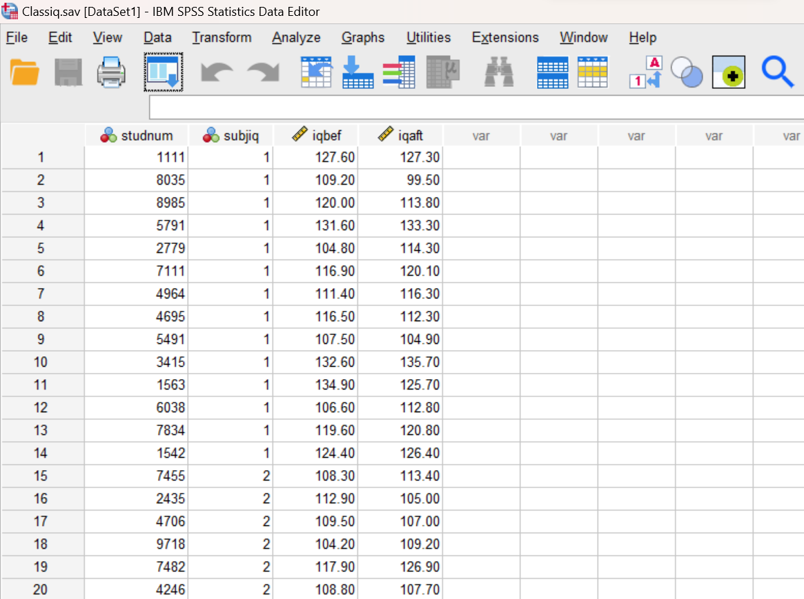
Examine Your Variables

Remember that before you proceed with any data analysis, you should always make sure that your variables are defined correctly. As you have learned in the previous labs, variable types are indicated by the icon to the left of each name, and additional information for variables can also be found by switching into the Variable View in your Data Editor. We will not be using the studnum (Student number) or subjiq (Subjective IQ) variables in this lab, so let’s just ignore those for now. Moving on to the other two variables, you should notice a ruler icon next to these indicating that they are designated as scale (continuous) variables. This is the correct variable type for variables to be compared in a paired samples t-test, so nothing more to do at this time.

Compute Descriptive Statistics

A good starting point for any analysis is to generate descriptive statistics for the variables you will be working with. In this case, let’s take a closer look at the iqbef (IQ before third grade) and iqaft (IQ after third grade) variables.

Since these are continuous variables, the DESCRIPTIVES command is appropriate. Open a Syntax Editor window (File→New→Syntax) and then type the following command. Or if you prefer, you can run the command through the SPSS menu system (Analyze→Descriptive Statistics→Descriptives and move both variables into the Variables box).

Review the results of the DESCRIPTIVES command in your Statistics Viewer window. Be sure you can find the mean and standard deviation for each of the two variables in the resulting output.

Annotate Your Output

Insert some text into your Statistics Viewer window at this point to describe the results of the descriptive statistics for our two variables of interest. Report the mean and standard deviation for each variable. What do you notice when you compare the two means? Remember to write your comments out in complete sentences, and try to use APA style (see Reporting Descriptive Statistics in APA style).

Paired Samples t Test

Although descriptive statistics such as these can provide some useful information, we can’t stop there! The principal’s hypothesis must be examined statistically by using a paired samples t-test in SPSS. The paired samples test is appropriate here because we are comparing pairs of scores (IQs before and after 3^rd grade) for the same group of children.

As with the other two versions of the t-test that we learned in the previous labs, we will use the T-TEST command to run the paired-samples t test. The PAIRS subcommand is used to request a paired samples test and to specify which variables are to be compared.

Return to your Syntax Editor window now (or open a new one if you haven’t already) and type the following statement to request the paired samples t-test:

Run the command and examine the output in your Statistics Viewer window. It should look similar to what is shown below. You should notice that this command produces four tables. The first table shows descriptive statistics for your two dependent variables, the second shows the correlation between these two variables, the third shows the results of the hypothesis test, and the fourth shows the effect size for your statistical test.

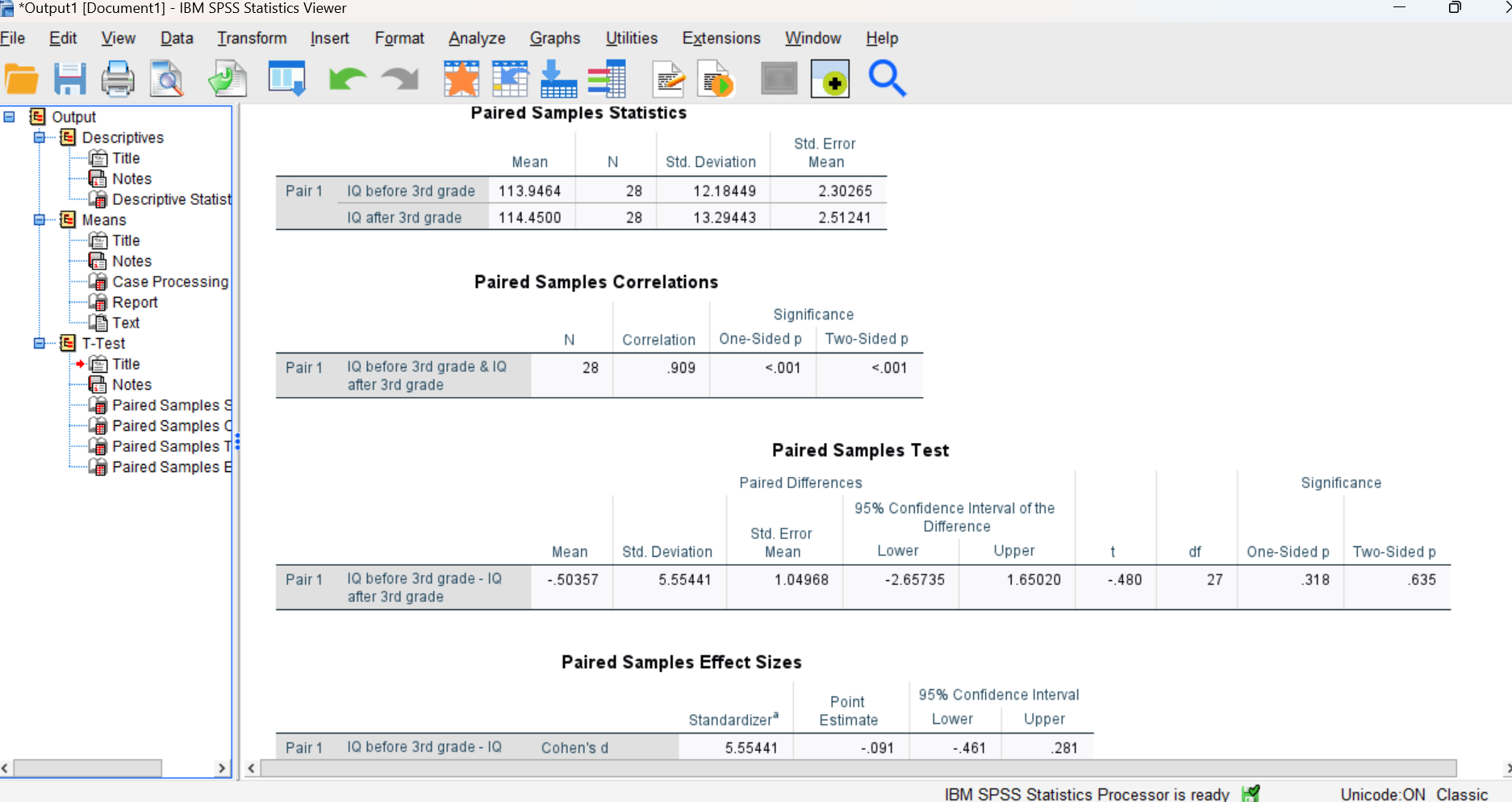
You can ignore the second table for now (you can actually delete it from your output if you want) since we’re not quite ready to discuss correlational analysis at this time. But stay tuned, we’ll get there in a future lab!

Directional vs. Non-Directional Hypothesis Tests

Up until this point in the class, we have been using the Two-Sided p value to evaluate the results of our hypothesis tests. It is appropriate to use the Two-Sided p value when we are performing a non-directional test, which means we are just testing to see if there is a difference between the two measures and we don’t have a prediction about which one should be larger. Non-directional tests are often referred to as “two-tailed” tests.

But for this lab, remember that the principal did have a prediction about the direction of the difference. In particular, she predicted that IQ scores after 3^rd grade would be higher than the IQ scores before 3^rd grade. So, in this case we should be performing a directional hypothesis test and using the One-Sided p value to make our decision about the null hypothesis. Directional tests are often referred to as “one-tailed” tests. As you can see in the third table (and is generally the case), the One-Sided and Two-Sided p values are different. So it is important to choose the correct one!

Determine your conclusion about the principal’s hypothesis by comparing your One-Sided p value to an alpha of .05. In this case we are actually testing the null hypothesis which states that the IQ scores after 3^rd grade are not higher than the IQ scores before 3^rd grade. The One-Sided p value must be less than your alpha level in order to reject the null hypothesis. If we reject the null, then of course we would have statistical support for the principal’s hypothesis.

Annotate Your Paired Samples t-Test Results

Insert several sentences into your output file at this point interpreting your results from the paired samples t-test. Again, let’s add some organization to your discussion of the results as we have done in the previous two labs. Report the information in the following order, and include the letters shown (A, B, C, and D) so each piece is clearly identified in your annotation:

1. Report the two sample means being compared (you will have to look in the first table to find those), t-value, degrees of freedom, and p value for your hypothesis test.
2. State your “statistical conclusion” about the null hypothesis – which is either to reject or fail to reject, and why you made that decision.
3. Report your Cohen’s d value (which you can find in the third table, use the Point Estimate) as well as your interpretation of the size of the effect. Remember to use the guidelines for Cohen’s d:

D. Finally, summarize all of that data gathering by writing an APA-style statement with your “real-world” conclusion about the 3rd graders’ IQ scores and the principal’s hypothesis. Was there a significant increase in IQ scores during 3rd grade as the principal predicted? Remember to include the means and standard deviations of each group, your conclusions about significant/not significant and higher/lower/the same when looking at the means, and the t-statement; see the examples that were given for the independent samples t-test in Lab #6 as paired samples t-tests are reported in the same way!

Another Paired Samples t Test

Use SPSS to complete the following exercise (from Levin & Fox, 2000).

Note: This exercise requires that you type a new set of data into SPSS. To type in new data, you will need go to your Data Editor window, click on File, then New, then Data (i.e., File→New→Data). As a result of this command, SPSS will create a new data window for you. Feel free to close the previous data window containing the Classiq data (and no need to save), we will not be using that data again in this lab. Do this now, and then continue with the following steps.

1. Define your two variables first (Variable View tab) and then enter the data (Data View tab) in your Data Editor window. Remember that SPSS variable names are restricted to a single word, but you should add variable labels to give lengthier descriptions.
2. Generate some appropriate descriptive statistics using the DESCIPTIVES command as we did earlier for the Classiq data.
3. Run a paired samples t-test to determine whether aggression has been reduced as a result of the conflict-resolution program. Please use this opportunity to run the test using the SPSS menu system (Analyze→Compare Means and Proportions→Paired-Samples T Test). In the Paired-Samples T Test dialog box, you will need to move your two variables to the first Pair in the Paired Variables list as shown here:

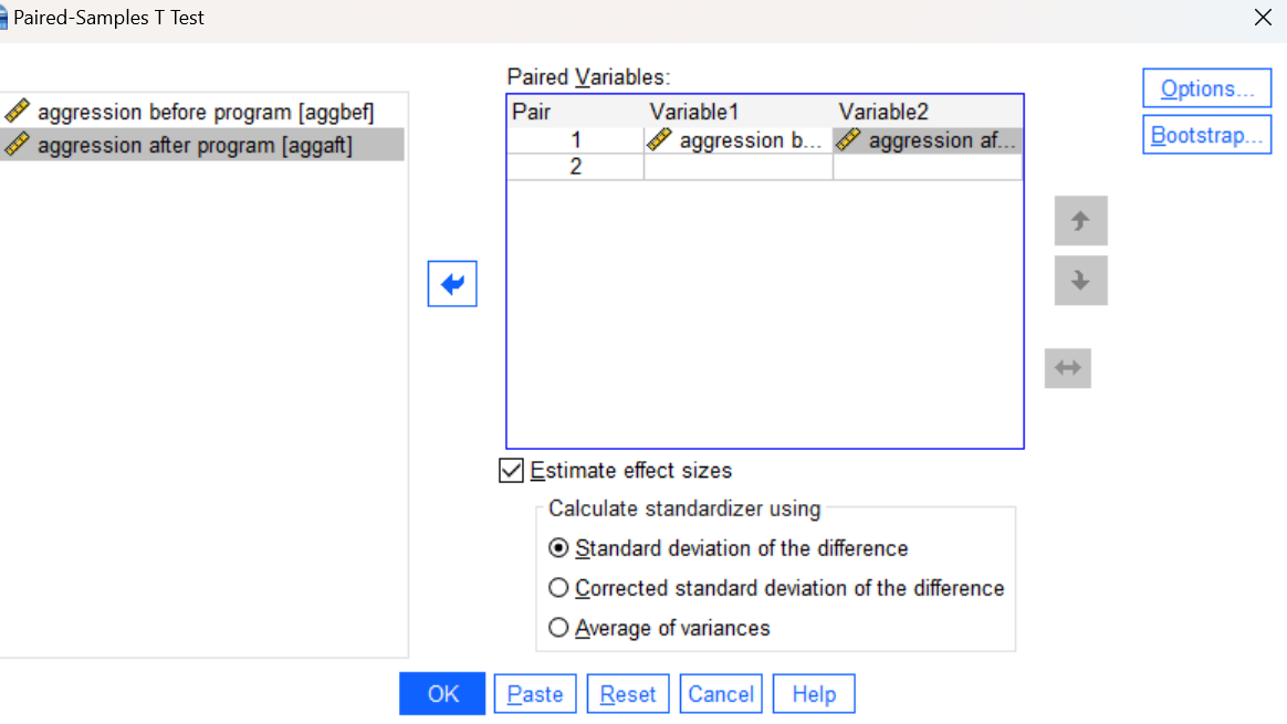
Press the OK button to run the command and review your results in the Statistics Viewer window.

Annotate Your Paired Samples t-Test Output

Again, insert comments into your output file at this point interpreting your results from the paired samples t-test. Follow the same instructions as for your previous annotation (including the A, B, C, D structure and labeling). When interpreting your output, remember to choose correctly between the One-Sided and Two-Sided p values and clearly state which one you are using to make your statistical decision about the null hypothesis. Was the Center for the Study of Violence correct in their prediction that the conflict resolution program would reduce aggressive behavior?

Insert Your Name

Insert your name and Lab #7 at the top of your statistical output as an identifier. See the previous Laboratories or ask a lab assistant if you need instructions.

Clean Up Your Statistical Output

Take a few minutes now to examine and clean up the contents of your Statistics Viewer window. When you are done it should include only the following outputs along with your annotations:

• Output of Descriptives command for iqbef and iqaft
• Paired samples t-test for iqbef vs. iqaft
• Output of Descriptives command for aggression data
• Paired samples t-test for aggression data

Save Your Work and Exit SPSS

Save the contents of your Syntax Editor, Data Editor, and Statistics Viewer windows to files on your own personal drive or workspace on the network. When saving the aggression data, use a meaningful name for the file such as “aggression.sav”. Also use meaningful names (e.g., Lab 7) for your syntax and output files so that they can be identified with this week’s lab. Use the Print to PDF function or export to PDF function to save “all visible” output to a PDF version of your output file. Open your PDF file and check to make sure it contains all your outputs and annotations. You can then exit SPSS by selecting the Exit option from the File menu in the active SPSS window (File→Exit).

Submit Your Lab

Submit the PDF version of your completely annotated output file in the D2L Brightspace Assignments folder when you’re done. After uploading the file to Brightspace, open it from the assignments folder and check to make sure you have submitted the correct file..