Lab #6 Independent Samples t-Test

In this laboratory you will learn how to:

• Load an SPSS data file
• Display descriptive statistics for variables in a data set
• Compute and interpret an independent samples t-test

Introduction

In this lesson we will learn more about the use of SPSS to test research hypotheses. Remember that a research hypothesis is simply a prediction or “educated guess” about a pattern of results that will be found in the data. Oftentimes, this hypothesis involves a comparison of two conditions (e.g., method A vs. method B) or two groups (e.g., males vs. females). This type of hypothesis requires a two-sample statistical test. SPSS provides two-sample t tests for this purpose. As for most statistical tests, t-tests involve defining a null hypothesis (typically stating that there is no difference in the means) and then drawing a conclusion about the research hypothesis based on how well the null hypothesis is supported by the data. In this lab we will focus on one particular type of two-sample t-test: the t-test for independent samples.

For this laboratory, we will be using the SPSS data file called “hourlywagedata.sav”, which contains hourly wage data for a sample of 3000 nurses working in both hospital and office (clinic or doctor’s office) settings. Before beginning the lab, you will need to download a copy of this file from the SPSS Data Files section of this book or from our course area in D2L Brightspace.

Several pieces of information were collected for each nurse and recorded in the dataset using the following variables:

position  type of nurse (hospital or office)

agerange  age category (18-30, 31-45, or 46-65)

yrsscale   years of experience category (5 or less, 6-10, 11-15, 16-20, 21-35, or 36+)

hourwage  hourly salary

Our main interest in this lab will be to compare the hourly salaries for the hospital nurses vs. the office nurses.

Start SPSS and Load the Data

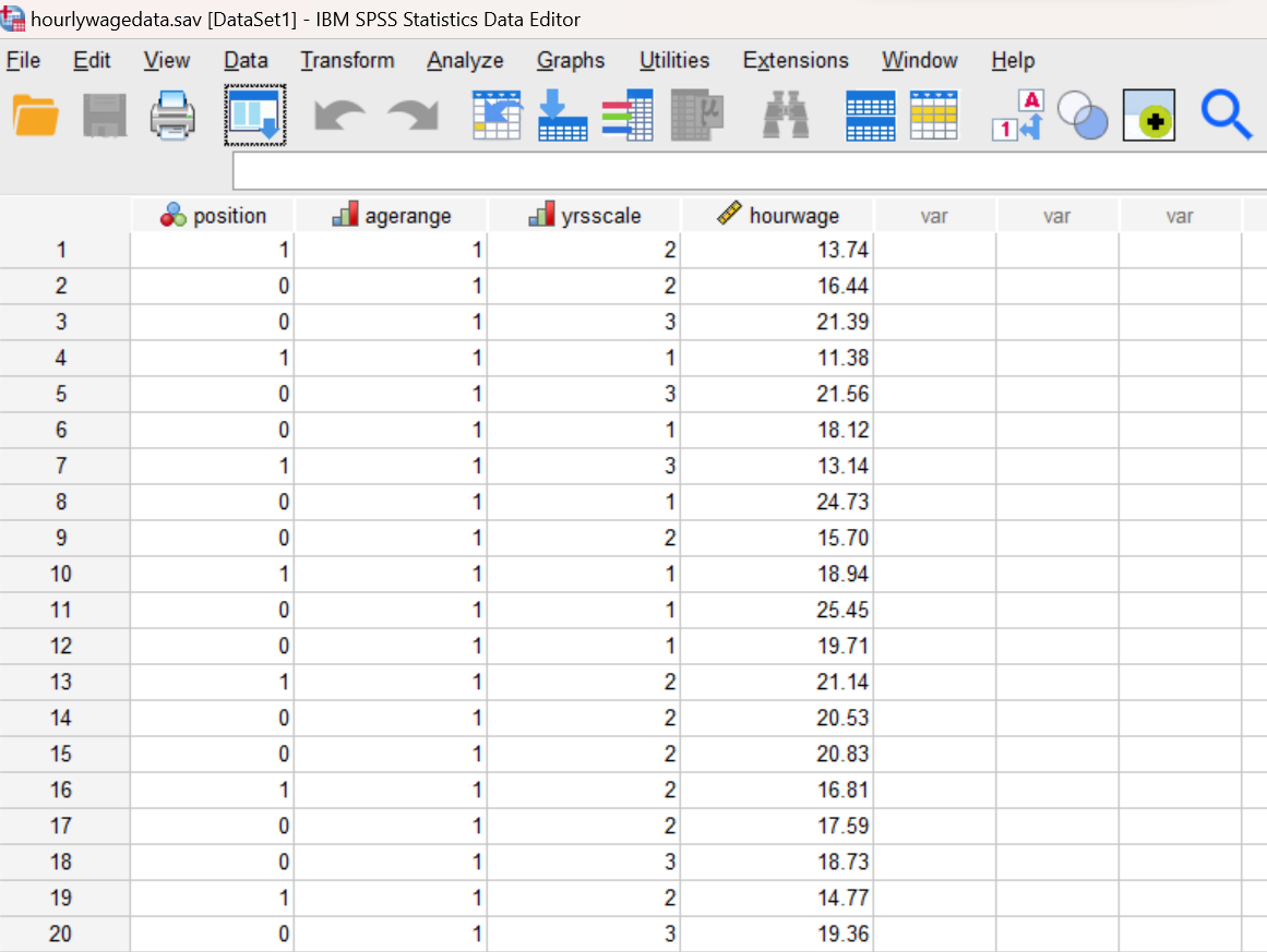
Start SPSS as you have done in previous labs, using your application menu or program search tool and load the hourly wage data into your Data Editor. At this point, your Data Editor window should be displaying the data as shown below:

Examine Your Variables

Click on the Variable View tab and examine your variables. You should notice that the position, agerange, and yrsscale variables are categorical (nominal or ordinal), whereas the hourwage variable is defined as a scale variable. Examine the information in the Values column and take note of the numeric value labels used for each of the defined categories for each of the three categorical variables. This is important information that you will need to know later when we run the independent samples t-tests for this lab.

Compute Descriptive Statistics for Categorical Variables

As you have learned by now, a good starting point for any analysis is to generate descriptive statistics for the variables you will be working with. Let’s start by generating some frequency distribution tables and barcharts (showing percentages) for our three categorical variables. Use Analyze→Descriptive Statistics→Frequencies to generate the output for position, age ranges, and years of experience from the menu system, or open a new Syntax Editor window (File→New→Syntax) and run the following command:

Review the results in your Statistics Viewer window.

Annotate Your Frequencies Output

Insert some text into your Statistics Viewer window at this point to describe the distribution of nurses for each of these variables. Write at least one complete sentence for each of the three variables, reporting frequencies and percentages. Try to write things out in APA style (see Reporting Descriptive Statistics in APA style).

Compute Descriptive Statistics for Continuous Variable

Now let’s take a closer look at our continuous variable hourwage (hourly salary). We could run the Frequencies command again for this one, but remember that a histogram is more appropriate for analyzing continuous variables (as opposed to the frequency distribution table). You can create a histogram for the hourwage variable in one of two ways: either use the Frequencies command in the Analyze menu (Analyze→Descriptive Statistics→ Frequencies) but turn OFF (de-select) the Display frequency tables option and use the Charts button to request a histogram OR use the Graphs menu (Graphs→Histogram).

Annotate Your Frequencies Output

After generating the histogram, insert some text into your Statistics Viewer window to describe the distribution of hourly salaries. Remember that when describing a histogram, it is good to mention the range of the data as well as the overall shape (i.e., symmetric or skewed) and location of any peaks in the distribution. Notice that SPSS also displays a mean and standard deviation when generating a histogram so we have those statistics too without generating them separately via other commands. Report those two statistics as part of your annotation.

More Descriptives for Continuous Variable

Because we’re interested in the hourly salaries across the two groups of nurses defined by the position variable, the MEANS command would be another good choice for descriptive statistics. Use the SPSS menu system to run the command using Analyze→Compare Means and Proportions→Means. Put the hourwage variable in the Dependent list (the outcome variable for which we want the means) and the position variable in the Independent List (the variable that creates the groups). You can also run this same analysis using the Syntax Editor if you prefer, with the following command:

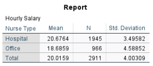
Review the results of the MEANS command in your Statistics Viewer window. Note that the second table (shown below) contains the overall mean for the sample (Total) as well as the means broken down by position (Hospital vs. Office).

Annotate Your Examine Output

Insert some text into your Statistics Viewer window at this point to describe the output you have just produced, and give your interpretation of the results. Clearly report the overall mean for the hourly salary data as well as the mean hourly salary for each of the two groups, with standard deviations. How do the means compare for the two types of nurses? One might predict that hospital nurses would earn higher salaries than office nurses. Does this prediction seem to be supported by the data? Explain.

Independent Samples t Test

Comparing the means for the two groups is a good starting point in determining whether there’s a difference. However, you must remember that if these are sample means, there is a margin of error surrounding each mean that must also be taken into account when making this kind of comparison. We could get 95% Confidence Intervals through an Explore/Examine command to assess the sampling error as we’ve done in previous labs, but we won’t do that here. Instead, another way to see if we actually have a statistically significant difference between the two groups is to use a t-test. The independent samples version of the t-test is appropriate here because we want to compare hourly salaries across two different groups of individuals (hospital nurses vs. office nurses) and it is reasonable to assume that one group’s hourly salaries have no relationship to the salaries in the other group (i.e., the samples are independent). The appropriate command in SPSS is called T-TEST.

Return to your Syntax Editor window (or open a new one if you haven’t already opened one) and let’s use the T-Test command to run an independent samples t-test. The command syntax is as follows:

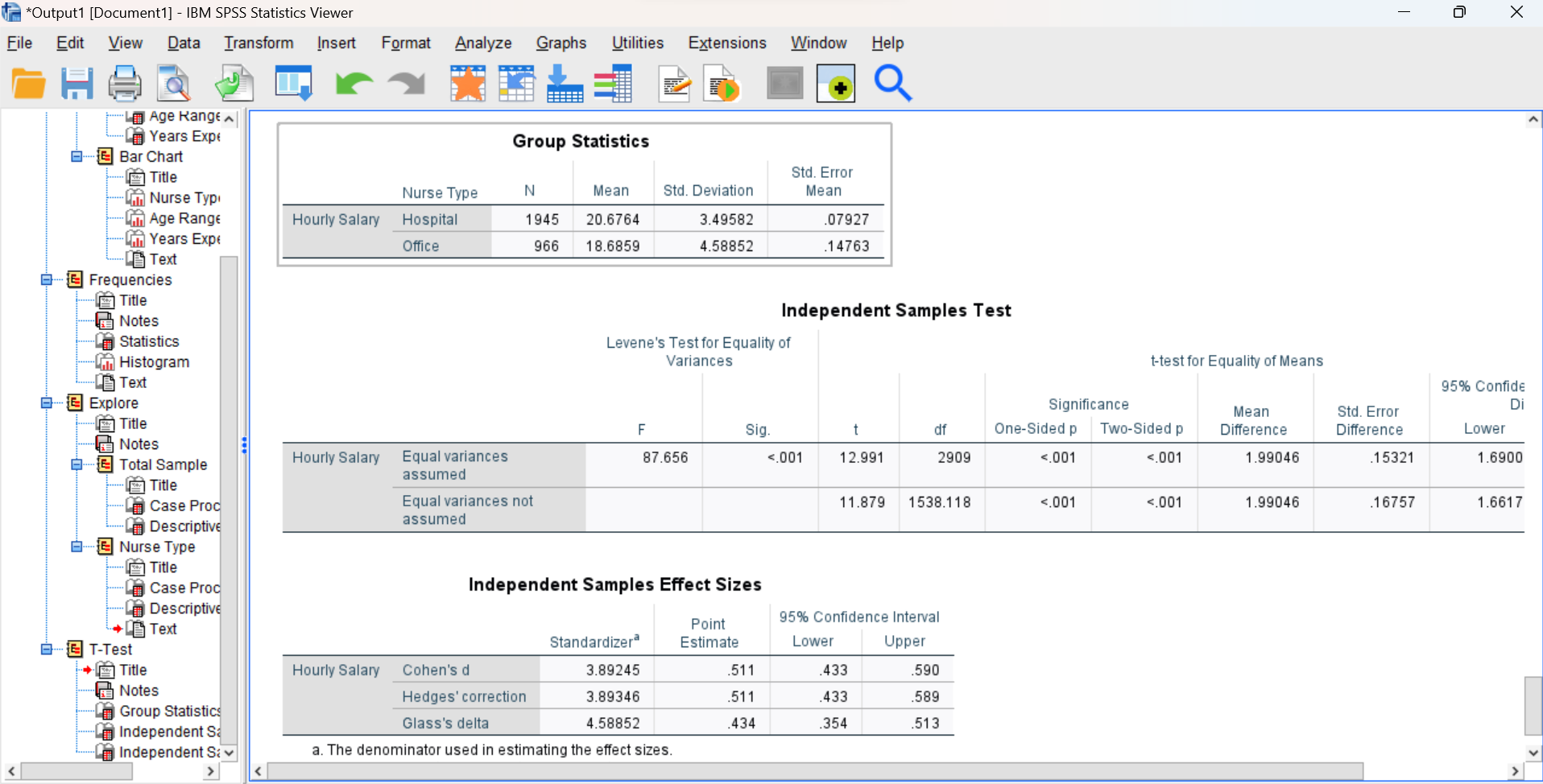
Run the command and examine the output in your Statistics Viewer window. It should look similar to what’s shown below. You should notice that this command produces three tables, very similar to what we saw for the one sample t-test in the previous lab. The first table shows descriptive statistics for your dependent variable within each of the two groups (similar to what the MEANS command gave you), the second shows the results of the hypothesis test, and the third shows the effect size for your statistical test.

Interpreting Hypothesis Test Results

In looking at the second table showing the hypothesis test results, your goal is to determine whether you can reject the null hypothesis. Remember, with the independent samples t-test we are actually testing the null hypothesis that the means for the two groups do not differ statistically. So, if you reject the null, you are concluding that there is a statistical difference between the two group means.

Interpreting Levene’s Test

As you can see in the second table, SPSS actually reports two different versions of the independent samples t-test, one for Equal variances assumed (top row) and the other for Equal variances not assumed (bottom row). The row to use depends on the results of Levene’s Test for Equality of Variances, which is reported in the left portion of the table as highlighted below:

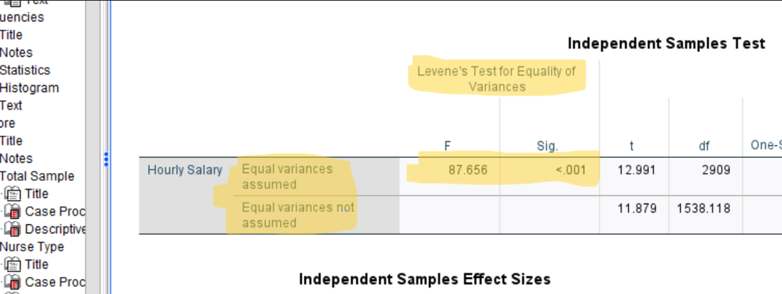
The purpose of Levene’s test is to determine whether the assumption of homogeneity (equality) of variances is satisfied. This is an important assumption, and if it is not satisfied, we need to use a different version of the independent samples t test. To determine whether the assumption is satisfied, you will need to look at the Levene’s test Sig. level (or more commonly referred to as the “p value”).

If the p value for Levene’s test is less than .05, we will conclude that the homogeneity of variances assumption is not satisfied. In other words, the variances of the two groups are not equal and we should use the version of the t-test adjusted for unequal variances (Equal variances not assumed row).

If the p value for Levene’s test is greater than or equal to .05, we will conclude that the homogeneity of variances assumption is satisfied. In this case we would use the standard version of the t-test (Equal variances assumed row).

For this particular test, Levene’s test produced a p value < .001, which is certainly less than .05. Thus, the homogeneity of variances assumption is NOT satisfied, and we should use the Equal variances not assumed (the bottom row of the table) to interpret the independent samples t-test.

Annotate Your Levene’s Test Results

Insert some comments into your Statistics Viewer window to report the results of Levene’s test. You should include a report of the Levene’s test p value as well as a statement indicating whether you will be using the equal variances or unequal variances version of the t-test for equality of means.

Interpreting Hypothesis Test Results (cont.)

Now, locate the portion of the second table containing results of the independent samples t-test. As we learned for the one sample t-test in the previous lab, we will be making our decision about the null hypothesis by examining the p value, and by using the rule that the p value must be less than the alpha level (.05) in order to reject the null. Again, let’s focus on the Two-Sided p value for now. Remember: if the p is low (< .05), then the null hypothesis “must go” (is rejected). If the p is not < .05, then you fail to reject the null hypothesis.

Annotate Your Independent Samples t-Test Results

Insert several sentences into your output file at this point interpreting your results from the independent samples t-test. As for the one sample t-test, there’s a lot of information to report, so let’s add some organization. Report the information in the following order, and include the letters shown (A, B, C, D) so each piece is clearly identified in your annotation:

1. Report the two sample means (you will have to look in the first table to find those), t-value, degrees of freedom, and p value for your hypothesis test. Make sure to use the correct row in the second table (based on the Levene’s test) for the t-test values!
2. State your “statistical conclusion” about the null hypothesis – which is either a reject or a fail to reject, and why you made that decision.
3. Report your Cohen’s d value (which you can find in the third table, use the Point Estimate value) as well as your interpretation of the size of the effect. Remember to use the guidelines for Cohen’s d, same as those given in the previous lab:

   d = 0.2	small effect
   d = 0.5	medium effect
   d = 0.8+	large effect

4. Finally, summarize all that data gathering by writing an APA-style statement with your “real-world” conclusion about the nurses’ hourly salary data. Was there a significant difference in salaries for hospital nurses as compared to the office nurses? If so, which group had higher salaries? Remember to include the means and standard deviations of each group, your conclusions about significant/not significant and higher/lower/the same when looking at the mean differences, and the t-statement. (See the Lab 6 Preview chapter for some examples of APA-style statements.)

Independent Samples t-Test Comparing Age Groups

Now, let’s repeat this process one more time but this time instead of comparing the salaries for hospital nurses vs. office nurses, let’s compare salaries for nurses in different age categories as defined by the agerange variable. And this time, let’s run the command using the SPSS menu system rather than typing in the command syntax.

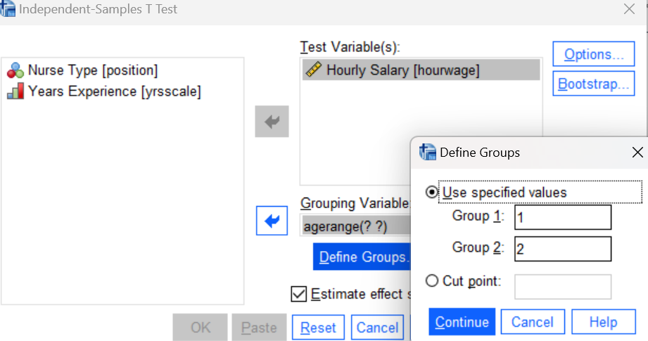
You can find the independent samples t-test in the Analyze menu, under Compare Means (Analyze→Compare Means and Proportions→Independent Samples T Test). Navigate to this command now, and in the resulting dialog box, move your hourwage variable to the Test Variable list and your agerange variable to the Grouping variable box as shown below. Importantly, you will also need to click on the Define Groups button and tell SPSS which age groups you would like to compare. Let’s use the values 1 and 2 here, which are the value labels for the 18-30 and 31-45 age groups, respectively (which you can see in the Variable View for the dataset as pointed out earlier).

After defining your groups, press the OK button to run the command and then examine the results in your Statistics Viewer window. Here again, SPSS will produce those three tables for the t-test as you saw earlier.

Annotate Your Independent Samples t-Test Output

Insert several sentences into your output file at this point interpreting your results from the independent samples t-test. When interpreting your output, remember to examine the results of Levene’s test first so you know whether to use the version of the t test that assumes equal variances or the one for unequal variances. Follow the same instructions as for your previous two annotations: the one for Levene’s test (can we assume equal variances or not and why) and the one for the independent samples t-test results (including the A, B, C, D, structuring of your reporting). So this annotation should include a complete and comprehensive analysis of your test results. One might assume that the older nurses are earning higher salaries because they have more years of experience. Is this assumption supported by the data?

Additional Practice (optional)

If you are interested, and would like more practice, go ahead and run some additional age group comparisons. For example, you could compare the 18-30 year-olds with the 46-65 year-olds by using the values 1 and 3 in your Define Groups dialog box. Or you could use the values 2 and 3 to compare the 31-45 year-olds with the 46-65 year-olds. Add some comments into your output file to describe the results of any additional analyses that you run; you can make those comments in any format you’d like to (this part of the lab is just for practice and will not count toward your lab score).

In case you’re wondering, yes, it is possible to run all of the pairwise comparisons at once when there are multiple groups defined by a categorical variable such as agerange. But not with the independent sample t-test, which is limited to just two groups at a time. There’s a different SPSS command for running multiple comparisons, which we will learn about in a future lab, so stay tuned!

Insert Your Name

Insert your name and Lab #6 at the top of your statistical output as an identifier. See the previous Laboratories or ask a lab assistant if you need instructions.

Clean Up Your Statistical Output

Take a few minutes now to examine and clean up the contents of your Statistics Viewer window. When you are done it should include only the following outputs along with your annotations:

• Frequency tables and bar charts for position, agerange, and yrsscale variables
• Histogram for hourwage variable
• Means command output for hourwage by position
• Independent samples t-test for hourwage by position
• Independent samples t-test for hourwage by agerange (comparing first two age categories)
• Optional additional independent samples t-test(s) comparing other age categories

Save Your Work and Exit SPSS

Save the contents of your Syntax Editor and Statistics Viewer windows to files on your own personal drive or workspace on the network. Give them meaningful names (e.g., Lab 6) so they can be identified with this week’s lab. Use the Print to PDF function or Export to PDF to save all visible output to a PDF version of your output file. Check that your saved PDF file contains all the required outputs and annotations, including your name and lab number at the top of the file. (No need to save your Data Editor contents since we did not make any changes to the data file.) Exit SPSS by selecting the Exit option from the File menu in the active SPSS window (File→Exit).

Submit Your Lab

Submit the PDF version of your completely annotated output file in the D2L Brightspace Assignments folder when you’re done. After uploading the file to Brightspace, open it from the assignments folder and check to make sure you have submitted the correct file.