Lab #8 Preview
One-way Analysis of Variance (ANOVA)
Purpose
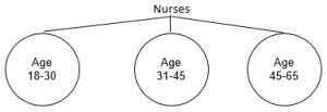
In this lab we will be comparing mean hourly salaries for nurses across three different age groups (illustrated below) and also for nurses with different years of experience. Do the salaries differ across the groups?

Grouping Variables (IVs/Factors):
- agerange = three age categories used in first analysis
- yrsscale = six categories of years of experience used in second analysis
Measures (DVs):
- hourwage = hourly salary
Null Hypothesis: There are no differences among the group means
Alternative Hypothesis: There is at least one difference among the group means
Levene’s Test is a preliminary test to determine whether the groups have equal variances.
ANOVA F test is a test of the null hypothesis. Based on test results, we either:
- Reject the null hypothesis (and conclude there is a mean difference somewhere among the groups), or
- Fail to reject the null hypothesis (and conclude none of the group means differ significantly)
Important: If the F test is significant, then post-hoc tests are performed to locate the significant difference(s). We will use the Tukey post-hoc test for this lab.
APA Style
APA style has a standard way to report hypothesis testing results. An ANOVA is reported like t-tests except that you typically have more than two group means (and standard deviations) to report and compare, and you write an F-test statement instead of a t-test statement.
Generally, as before, you report whether the results were “significant” or “not significant”, and make conclusions about means being smaller, bigger, not different, etc. for your analysis. This often takes more wording than with a t-test because you have multiple comparisons of means to describe and explain, although you only have to report the value for each mean (and SD) once even though you might describe how a group compares to multiple other groups. With many groups, a researcher might decide to report the means in a table rather than in the text.
The F-statement is reported in a similar format as the t as well (with df, the calculated F, p value, and effect size). However, F-tests have two different degrees of freedom which are reported in parentheses with a comma between them: F(#dfbetween, #dfwithin) = xxx. [dfbetween is the number of groups minus one (k – 1) and dfwithin is the total number of people minus the number of groups (N – k).]
Some examples (with made up numbers) are given below. You might see something like the following to report a one-way ANOVA in APA style.
With no group differences (overall ANOVA not significant):
- The average intelligence did not differ by major, F(2, 48) = 1.63, p > .05, η2 = .02. The mean for science majors of 111.25 (SD = 15.2), the mean for social science majors of 110.75 (SD = 12.6), and the mean for humanities majors of 109.82 (SD = 14.5) did not differ significantly.
With group differences between some of the means (overall ANOVA significant): look for patterns if not all pairs of means are different (e.g., these two means are the same and are lower than the third mean) and describe those patterns. Putting M and SD in parentheses (as with the second example here) often simplifies the text needed to describe the effects, but it can be trickier to write with proper grammar this way. Remember that if you can read the sentence just fine while omitting all of the information in parentheses then you have used parentheses grammatically correctly, but if you need to SAY any of the information in parentheses in order to read the sentence, then that information should not be in parentheses.
- The effect of dosage on reaction time was significant, F(2, 26) = 8.76, p = .012, η2 = .08. A Tukey’s post-hoc test examined the differences in means. The participants in the high dosage group had an average reaction time of 12.3 seconds (SD = 4.1), which was significantly longer than both the moderate dosage and control groups. The participants in the moderate dosage group, with an average reaction time of 7.4 seconds (SD = 2.3), and the participants in the control group, with an average of 6.6 seconds (SD = 3.1), did not differ significantly.
- The height of female athletes was significantly different by sport, F(4, 345) = 7.87, p < .001, η2 = .18. Post-hoc tests revealed that basketball players (M = 71.3 inches, SD = 3.4) and volleyball players (M = 70.5 inches, SD = 4.2) were equal in height and the track athletes (M = 64.8 inches, SD = 3.6) and soccer players (M = 65.9 inches, SD = 3.9) were equal in height. However, the basketball and volleyball players were significantly taller than the track and soccer players.
