
Lab #10 Chi-Square Tests
Watch this RStats video for a good discussion of how to perform and interpret a chi-square goodness of fit test in SPSS. We will be running this kind of test in the second part of the lab. Note: if the video doesn’t play here, click the link to Watch on YouTube.
In this laboratory you will learn how to:
- Enter a summary table of frequencies into SPSS
- Compute and interpret a chi-square test for independence
- Compute and interpret a chi-square goodness of fit test
Learning Objectives
This laboratory addresses the following course objectives:
- Perform basic file operations in SPSS.
- Use SPSS to compute basic descriptive statistics.
- Use SPSS to perform common statistical tests.
- Execute SPSS commands using syntax editor and menu system.
- Interpret SPSS outputs.
Introduction to Chi-Square
In many research scenarios, data are collected using nominal or ordinal scales of measurement where participants are simply placed into categories defined for variables such as gender, class standing, or major in school. The data of interest to the researcher are frequencies within the various categories. Since these types of measures are not numerical, it is impossible to compute means and standard deviations, and thus the data cannot be analyzed using the standard t-test or analysis of variance approaches. While some forms of correlation analysis may be applicable (e.g., Spearman or point-biserial) for categorical data, it is more common to use an approach known as chi-square analysis (the Greek letter chi (Χ) is pronounced like “kai” or “kye”, rhymes with “sky”). In this laboratory we will examine two types of hypothesis tests for frequency data that are based on the chi-square distribution.
The chi-square test for independence is used to determine whether there is a relationship between two variables of interest. The chi-square goodness of fit test is used to determine how well a sample frequency distribution fits a specific population distribution.
We will be using the SPSS data file “train.sav” in the first part of this laboratory. You will need to download this file from the SPSS Data Files section of this book or from our course area in D2L Brightspace. These data are from a hypothetical training experiment, in which two different training methods were implemented to improve performance on a complex task. Participants were given a pretest to measure their baseline performance on the task and then randomly assigned to one of the two training methods. After six hours of training, the participants were tested again using a posttest. Most importantly for this lab, the participants were also questioned after the training session to determine their opinions about the training. One of the questions they were asked was whether they thought the task was boring (Yes or No). The experimenter wanted to test several things:
- He wanted to compare the pretest scores to posttest scores for all participants to see if the training actually improved performance. He hypothesized that training of any kind would be likely to improve performance.
- He wanted to compare the results of the two training methods. He believed the first training method would prove to be superior.
- He wanted to know whether there was a difference in the number of people who found the task boring for the two training methods. He thought that people might find one method more boring than the other.
While t-tests could be used to test the first two hypotheses, the third hypothesis involves categorical data and will require a different approach. In this laboratory, we will use the chi-square test for independence to examine the experimenter’s third hypothesis.
Start SPSS and Load the Data
Start SPSS as you have done in previous labs, using your application menu or program search tool and load the “train.sav” data file into your Data Editor. At this point, your Data Editor window should be displaying the data as shown below:
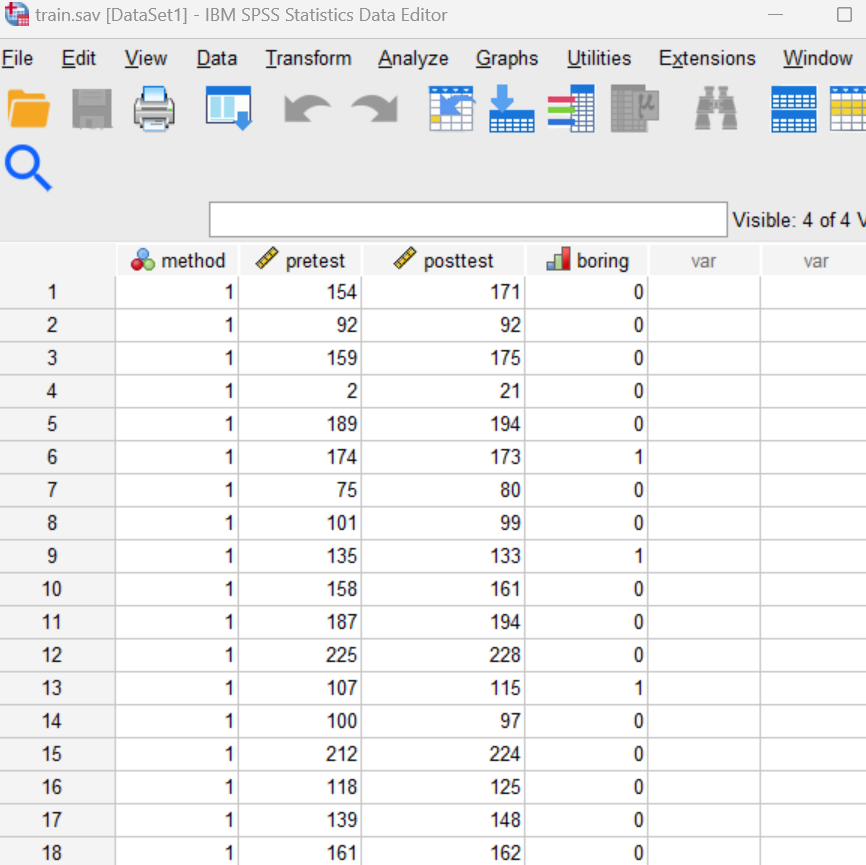
Examine Your Variables
Examine your variables in the Data Editor, both in the Data View tab and the Variable View tab. You should notice that the method and boring variables are categorical variables, whereas the pretest and posttest variables are defined as scale variables.
Chi-Square Test for Independence
The experimenter’s third hypothesis involves comparing the two training methods in terms of how boring the participants found the task. Since both variables of interest here (method and boring) are categorical, a chi-square test for independence can be used. Note that when using the chi-square test, we are really testing the null hypothesis that there is no relationship between the variables (in other words, that they are independent). If there is sufficient evidence to reject the null hypothesis, then we will conclude that there is a relationship between the variables (in other words, we will conclude that they are not independent).
The CROSSTABS command can be used to show the number of observations in each category and also to request the chi-square statistic (CHISQ). Open a Syntax Editor window (File→New→Syntax) and type the following command:
CROSSTABS
/TABLES method BY boring
/STATISTICS = CHISQ.
The TABLES subcommand tells SPSS how to set up the cross-tabulation. The variable before the BY keyword will be displayed on the rows of the table and the variable after the BY keyword will be displayed on the columns.
The STATISTICS subcommand is used here to request the chi-square test.
Run the command and examine the output in your Statistics Viewer window. Several tables are produced by this command. Let’s start by looking at the Crosstabulation table (shown below), which displays the frequency of Yes and No responses within each training group.
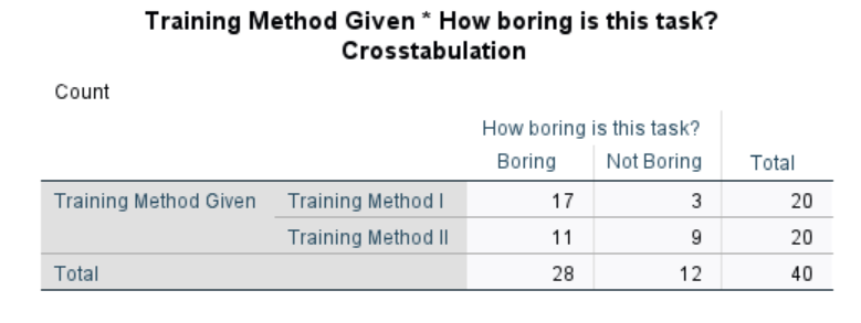
Annotate Your Crosstabulation Results
Insert some text into your Statistics Viewer window now to report the frequencies obtained for the Yes and No responses within each training group. Comment on which training method seems to be more boring for the participants based on these frequency data. (Note that since the total number of people using Method I and Method II are the same, 20 each, we can compare the counts of boring/not boring of each rather than turning the counts into percentages, which would be needed if the sample sizes for the two method groups were not the same.)
Interpreting the Chi-Square Test
Following the Crosstabulation table in your output file is a table of Chi Square Tests, which lists a number of different test statistics as shown here.
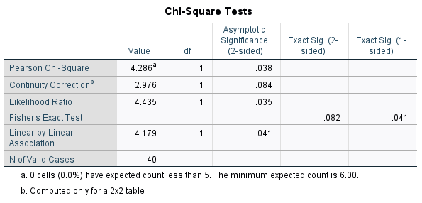
The test statistic we will be using is called the Pearson Chi-Square (first row of the table). If the value of this statistic is sufficiently large, then you can reject the null hypothesis and conclude there is a significant relationship between the two variables, in this case, that participants’ perception of how boring the training is depends on the training method. (In other words, it would tell us that the proportion of participants who find the training boring is significantly different for the two methods.)
The Asymptotic Significance (which is basically just another kind of p value) tells you whether the chi-square statistic is large enough to reject the null. If this p value is less than your alpha level (let’s use .05, as usual), you will reject the null hypothesis and conclude there is a significant relationship – meaning the variables are not independent of one another. If the p value is greater than your alpha level, you will fail to reject the null and conclude the relationship is not significant – meaning the variables are independent of one another.
Annotate Your Chi-Square Test for Independence Results
Insert some text into your Statistics Viewer window at this point to interpret the results of the chi-square test for independence. Please use the A and B labeling for your statements as indicated here.
- Report your statistical conclusion about the null hypothesis (reject or fail to reject, and explain why).
- Write your APA style statement about the results of the chi-square, following the standard examples shown in the Lab Preview document. You reported on the frequencies in your first annotation already but should repeat them here in a format that makes sense for APA style. After the frequency content, write your statement giving the conclusion about the significance (or lack thereof) of the chi-square test with the APA style chi-square statistics statement (including df, N, chi-square value, and p-value). Make sure your statement is clear about the “real-world” conclusion for the experimenter’s hypothesis.
Running Crosstabs from the Menu System
As you can probably guess, the Crosstabs command can also be run from the SPSS menu system. Crosstabs is available in the Analyze menu under Descriptive Statistics (Analyze→Descriptive Statistics→Crosstabs). Go ahead and navigate to this command now and see if you can produce the same results as you obtained using the command syntax. In the Crosstabs dialog box, you will need to move the two categorical variables to the Row and Column boxes as shown below:
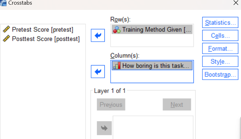
You will also need to click on the Statistics button and check the box to select the Chi-square test. Press the OK button in the Crosstabs dialog box to run the command and then review your results in the Statistics Viewer window. Once you have successfully reproduced the previous outputs, delete the duplicate tables from your output file and continue with the rest of the laboratory.
Chi-Square Goodness of Fit Test
To demonstrate the chi-square goodness of fit test, let’s consider the following problem. Historically, the grades in a particular course have been distributed with 20% A’s, 30% B’s, 30% C’s, 15% D’s, and 5% F’s. After switching to a new textbook for the course, the professor wants to determine whether the distribution of grades is the same as before or is different in some way. A sample of 200 students after the textbook switch yields the following data:
| Grade | Frequency |
| A | 50 |
| B | 75 |
| C | 55 |
| D | 17 |
| F | 3 |
Step 1: We need to start by entering the data. These data can be entered into SPSS either by using the raw data (200 observations!) or by using the WEIGHT command (a major shortcut!). We will use the WEIGHT command. Return to your Syntax Editor window and type the following command lines. Note that we are using 1 for ‘A’ grades, 2 for ‘B’ grades, etc. As you have probably learned by now, SPSS is very picky about spelling, punctuation, and spacing, so be very careful to type things exactly as shown here and double check your work before moving to the next step.
DATA LIST FREE /grade count.
BEGIN DATA.
1 50
2 75
3 55
4 17
5 3
END DATA.
WEIGHT BY count.
Step 2: Use your mouse to select and highlight all of these command lines and then press the green triangle icon at the top of your window to run them all at once. Note that the purpose of these commands is to enter some data into SPSS. This command will actually create a new Data Editor window.
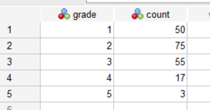
Step 3: Locate the new Data Editor window that is produced by the command and bring it to the forefront. If the command has been run correctly, you should see the data in your Data Editor window as shown below. As noted above, using the WEIGHT command is a different way to enter frequency data. These data do look different from what we are used to seeing; that’s because the data aren’t the raw data (which would be a list of 200 students’ grades entered as a 1-5) but a weighted count data set where the second column tells SPSS how frequent each grade is in the dataset. This setup works for chi-square because the frequency data is what we need to analyze.
Step 4: Now that the data are entered, we can perform the chi-square analysis. In this case, we will be performing a chi-square goodness of fit test to see if this sample distribution of grades differs from the historical grade distribution. The NPAR TESTS command is used for this type of chi-square test (note that NPAR refers to non-parametric). Return to your Syntax Editor window and type the following command lines:
NPAR TESTS
/CHISQUARE = grade(1, 5)
/EXPECTED = 20, 30, 30, 15, 5.
The CHISQUARE subcommand is used to request the chi-square goodness of fit test. The low and high values for the grade variable are given in parentheses after the variable name. Remember that we are using 1 for ‘A’ grades, 2 for ‘B’ grades, etc., so 1 is actually the “highest” grade of A and 5 is the “lowest” grade of F.
The EXPECTED subcommand is used to specify the expected percentages under the null hypothesis. These represent the percentages in the population grade distribution that we will be comparing the sample against. In this case we want to compare the current sample distribution of grades after the textbook switch to the historical grade distribution for the class where there were 20% A’s, 30% B’s, etc.
Step 5: Run the command and examine the output in your Statistics Viewer window. This command should produce two tables as shown here:
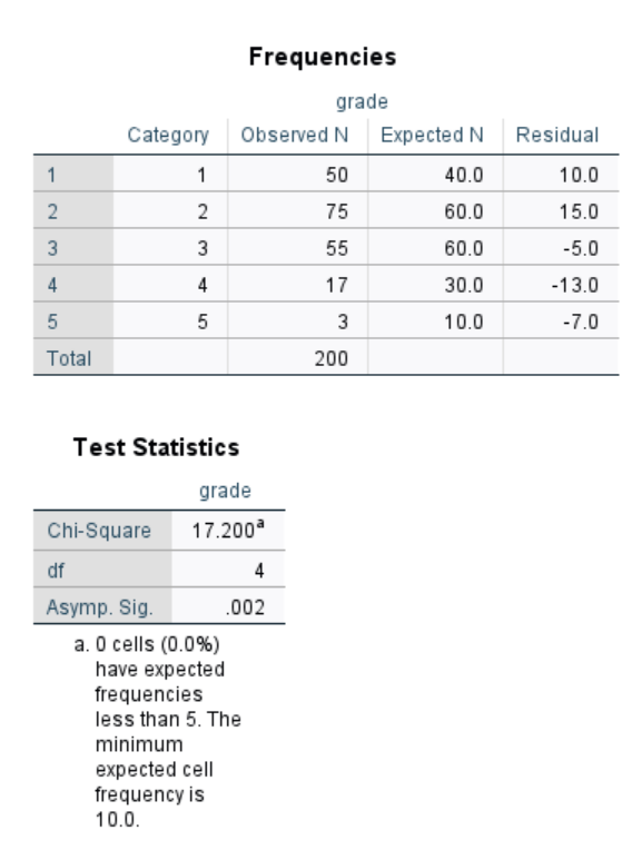 The first table shows a comparison of the observed (sample) frequencies versus expected frequencies, where the expected frequencies are computed based on the percentages you specified in the NPAR TESTS command. The Residuals are the differences between what was observed and what was expected.
The second table shows the results of the actual chi-square test. The null hypothesis for this test is that there is no difference between the observed and expected frequency distributions; that is, that the grade distribution after the new textbook (our observed data) would be the same as the historical grade distribution in the course (the expected frequencies). If the reported Asymptotic Significance (p value) is less than our alpha level (let’s use .05), we will reject the null hypothesis and conclude that the distributions are significantly different. If the reported Asymptotic Significance is greater than our alpha level, we will fail to reject the null hypothesis and conclude there is no significant difference between the distributions.
Annotate Your Chi-Square Goodness of Fit Test Results
Insert some text into your Statistics Viewer window at this point to interpret the results of the chi-square goodness of fit test. Again, please use the A and B labeling for your statements.
- Report your statistical conclusion about the null hypothesis (reject or fail to reject, and explain why).
- Write your APA style statement about the results of the chi-square test, following the standard examples shown in the Lab Preview document. Report the data on the frequencies of the grades in the course. After the frequency data, write your statement giving the conclusion about the significance (or lack thereof) of the chi-square test with the APA style chi-square statistics statement (including df, N, chi-square value, and p-value). Make sure your statement is clear about the “real-world” conclusion for the professor’s hypothesis; how would you address the professor’s question about the grade distribution obtained with the new textbook?
Running NPAR TESTS from the Menu System
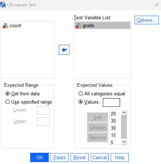
The chi-square goodness of fit test is available in the Analyze menu under Non-Parametric Tests (Analyze→Non-Parametric Tests→ Legacy Dialogs→Chi-Square). Go ahead and navigate to this command and see if you can produce the same results as you obtained using the command syntax. In the Chi-square Test dialog box, you will need to put grade in the Test Variable List and enter your set of expected percentages in the Expected Values box (in the same order as the grade category list) as shown below.
Press the OK button to run the command and then review your results in the Statistics Viewer window. Once you have successfully reproduced the previous outputs, delete the duplicate tables from your output file and continue with the rest of the laboratory.
Insert Your Name
Insert your name and Lab #10 at the top of your statistical output as an identifier. See the previous Laboratories or ask a lab assistant if you need instructions.
Clean Up Your Statistical Output
Take a few minutes now to examine and clean up the contents of your Statistics Viewer window. When you are done it should include only the following outputs and related annotations:
- Crosstabs and chi-square for method by boring
- Chi-square test comparing observed vs. expected grade distribution
Save Your Work and Exit SPSS
Save the contents of your Syntax Editor, Data Editor, and Statistics Viewer windows to files on your own personal drive or workspace on the network. If you want to save the file with your grade data, use a meaningful name such as “grades.sav”. Also use meaningful names (e.g., Lab 10) for your syntax and output files so that they can be identified with this week’s lab. Use the Print to PDF function or Export to PDF function to save all “visible output” to a PDF file. Exit SPSS by selecting the Exit option from the File menu in the active SPSS window (File→Exit).
Submit Your Lab
Submit the PDF version of your completely annotated output file in the D2L Brightspace Assignments folder when you’re done. After uploading the file to Brightspace, open it from the assignments folder and check to make sure you have submitted the correct file and it contains all the required items.