Lab #5 One Sample t-Test

In this laboratory you will learn how to:

• Load an SPSS data file
• Display descriptive statistics for variables in a data set
• Compute and interpret a one-sample t-test

Introduction

 

In this lesson we will begin to learn how to use SPSS to test research hypotheses. A research hypothesis is simply a prediction or “educated guess” about a pattern of results that will be found in the data. Sometimes, the research hypothesis involves comparison of a sample against a larger population having known characteristics (e.g., mean and standard deviation). This type of hypothesis requires a one sample statistical test such as the z-test. The z-test requires that we know both the mean and standard deviation of the population.

SPSS provides a more useful version of this test called the one sample t-test, which can be used even when the population standard deviation is unknown (which is often the case). As for most statistical tests, t-tests involve defining a null hypothesis (typically stating that the treatment has no effect) and then examining the data to see how well this null hypothesis is supported. As a result of the analysis, the researcher will either fail to reject the null hypothesis (and conclude the treatment has no effect) or reject the null hypothesis (and conclude the treatment does have an effect).

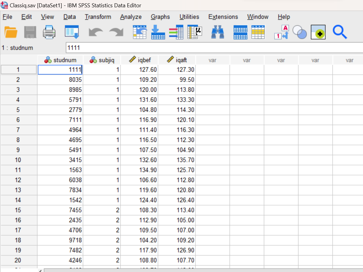
For this laboratory, we will be using an SPSS data file called “Classiq.sav”. These data are from a sample of third grade students at a private school. You will need to download this file from the SPSS Data Files section of this book or from our course area in D2L Brightspace. Several pieces of information were collected for each student. Of importance for this lab are the IQ scores measured for the students at the beginning (iqbef) and end (iqaft) of the third grade year.

The school principal would like to show that the intelligence level (as measured by IQ score) of the third grade students at her school is different from that in the general population where the mean IQ is known to be 100. Here, the “treatment” is the private school experience, and the null hypothesis would state that the private school experience has no effect on IQ scores. Please note that we are NOT comparing IQ scores before versus after third grade in this lab (we’ll look at that in a future lab). We just want to test whether the measured IQ scores (before and after third grade) are statistically different from what we would find in the general population.

Start SPSS and Load the Data

Start SPSS as you have done in previous labs, using your application menu or program search tool and load the Classiq.sav data into your Data Editor. Once you have done that, your Data Editor window should be displaying the data as shown below. Browse through the data a bit. How many third graders are included in this sample?

Examine Your Variables

Before analyzing the data, you should always make sure that your variables are defined correctly. As you learned in previous labs, variable types such as Nominal, Ordinal, and Scale are of particular importance because certain statistical functions require specific types of variables. In the Data Editor, the type of each variable is indicated by an icon to the left of the variable name. You can see by the ruler icon that the iqbef and iqaft variables are both designated as Scale (continuous) variables. The other two variables (studnum and subjiq) are designated as Nominal (categorical) variables. If you click on the Variable View tab in your Data Editor window you can see additional information for each of the variables in your dataset.

Compute Descriptive Statistics

A good starting point for any analysis is to generate descriptive statistics for the variables you will be working with. For this lab, we will only be using the iqbef (IQ before third grade) and iqaft (IQ after third grade) variables, so let’s take a closer look at those two variables now. Since these are Scale variables, the DESCRIPTIVES command is appropriate.

Use Analyze→Descriptive Statistics→Descriptives to analyze the data for both iqbef and iqaft from the menu system, or open the Syntax Editor window (File→New→Syntax) and run the following command:

Review the results of the DESCRIPTIVES command in your Statistics Viewer window. Locate the mean and standard deviation for each of our two variables of interest.

Annotate Your Descriptives Output

Insert some text into your Statistics Viewer window at this point to report the mean and standard deviation for the two variables. Also, write a statement about how the IQ scores of the 3^rd grade students in this sample seem to compare to the general population, which has a mean of 100 on intelligence.

One Sample t-Test for IQ Before 3^rd Grade

The principal’s hypothesis that her students have IQ scores different from those in the general population can be tested using a one sample t-test. An important component of the one sample t-test is a number called the “test value”. The test value is used to specify a comparison population mean. Note that this is the population mean that would be stated in the null hypothesis (if the private school has no effect on IQ, then the mean IQ score for 3^rd graders at the private school should be 100, just like in the general population). So, in this case, we want to compare our sample mean to a population mean of 100, and thus the test value should be 100.

To perform the t-test for IQ scores obtained before 3^rd grade, type the following in your Syntax Editor window (open a new Syntax window if you didn’t use syntax for the Descriptive analysis above):

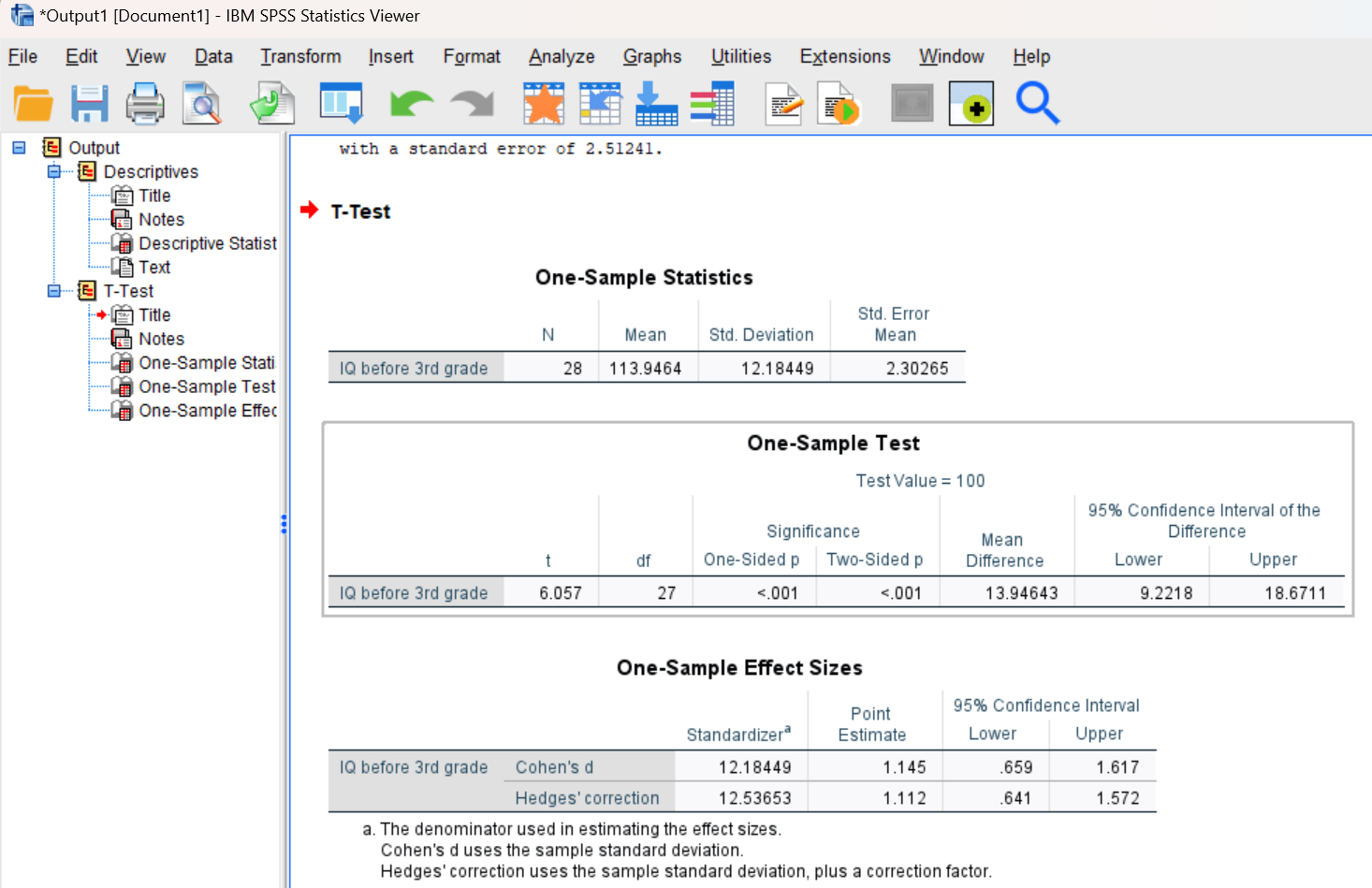
Run the command and examine the output in your Statistics Viewer window. It should look similar to what is shown below. You should notice that this command produces three tables. The first table shows descriptive statistics for your dependent variable (or variables; this will match what you already calculated above using the Descriptives command!), the second table shows the results of the hypothesis test, and the third shows the effect size for your statistical test.

Interpreting Hypothesis Test Results

The sample mean and standard deviation in the first table should be familiar from past labs. The standard error of the mean is also given; this statistic is used in the calculation for the t-test so it should be familiar from your stats lecture course (calculated as the standard deviation divided by the square root of n). Remember that standard error is a measure of sampling error.

In looking at the second table showing the hypothesis test results, you will find the calculated t-value, the degrees of freedom for the test (which for a one sample t-test is n-1), and the “significance”, which is the p value. The 95% confidence interval around the difference between the sample and population mean (where the null hypothesis would expect that mean difference to be zero) is also given, but we will not use that in this lab. Your goal is to determine whether or not you can reject the null hypothesis. Remember, with the one sample t-test we are actually testing the null hypothesis that the sample mean does not differ from the general population mean. So, if you reject the null, you are concluding that there is a statistical difference between the sample mean and the “test value”.

We generally make our decision about the null hypothesis by examining the p value, and by using the rule that the p value must be less than the alpha level (typically set at .05) in order to reject the null. You will notice that SPSS reports both a One-sided p value and a Two-sided p value. We’ll use the Two-sided p because our hypothesis as stated above is non-directional / two-tailed. (We will do more with one-sided and two-sided p values in a future lab.) If the p reported is < .05, we would reject the null for this particular hypothesis test; if the p is > .05, we would fail to reject the null. Remember from stats class that the p is the probability of this result happening if the null hypothesis is true; if the p value is small – this result would happen less than 5% of the time — that means the result would be rare if the null hypothesis is true, so then we make the conclusion that the null hypothesis is likely “not true” and should be rejected. Note that for very small p values, SPSS will just report them as “< .001”.

Interpreting Effect Size

SPSS produces a measure of effect size called Cohen’s d for the one sample t-test. Cohen’s d measures the size of the difference between the sample mean and the population mean in standard deviation units. Guidelines for interpreting Cohen’s d are as follows:

You can look in the third table to find Cohen’s d (look at the value in the Point Estimate column and don’t worry about Hedge’s correction for now) and compare that to the guidelines above to be able to claim that an effect (the difference between the sample and population means, in this case) is small, medium, or large. If Cohen’s d turns out to be a negative number, just take the absolute value (i.e., make it positive) before comparing to the above guidelines. For example, if the d was .61 (or -.61), we would call that a medium effect.

Annotate Your One Sample t-Test Output

Insert a few sentences into your output file at this point describing and interpreting your results from the one sample t-test. There’s a lot of important information to report, so let’s add some organization. Report the information in the following order, and include the letters shown (A, B, C, D) so each piece is clearly identified in your annotation:

1. State the sample mean (from descriptives table), t-value, and p-value for the hypothesis test
2. State your “statistical significance” conclusion – do you reject or fail to reject the null? – and how you made that decision
3. State Cohen’s d and your interpretation of the size of the effect
4. Write an APA style “real-world” conclusion statement about the principle’s hypothesis – state what you can conclude about the principal’s hypothesis and add the APA style “t-statement” at the end. (See the APA style examples given in the Lab #5 Preview chapter. This “real-world” conclusion statement will repeat some of the above information but put it into context with APA style.)

One Sample t-Test for IQ After 3^rd Grade

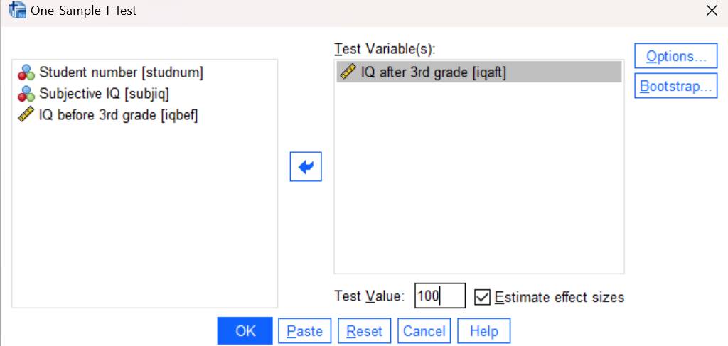
Now, let’s repeat this process one more time but this time using the iqaft variable (IQ scores measured after 3^rd grade) to see whether the IQ scores obtained after 3^rd grade different significantly from the general population mean of 100. And this time, let’s run the command using the SPSS menu system rather than typing in the command syntax.

You can find the one sample t-test in the Analyze menu under Compare Means (Analyze→Compare Means and Proportions→One Sample T Test). Navigate to this command now, and in the resulting dialog box, move your iqaft variable to the Test Variable list, and set the Test Value to 100 as shown below. Then press OK to run the command and examine the results in your Statistics Viewer window.

Annotate Your One Sample t-Test Output

Again, insert information into your output file for this new one-sample t-test analysis. Follow the same instructions and organization (A, B, C, D, format) as for your previous annotation. Are your results or conclusions any different now that we’re examining the IQ scores after 3^rd grade rather than before 3^rd grade?

Insert Your Name

Insert your name and Lab #5 at the top of your statistical output as an identifier. See the previous Laboratories or ask a lab assistant if you need instructions.

Clean up Your Statistical Output

Take a few minutes now to examine and clean up the contents of your Statistics Viewer window. When you are done it should include only the following outputs along with your annotations:

• Descriptive statistics for iqbef and iqaft variables
• One-sample t-test results for iqbef
• One-sample t-test results for iqaft

Save Your Work and Exit SPSS

Save the contents of your Syntax Editor and Statistics Viewer windows to files on your own personal drive or workspace on the network. Give them meaningful names (e.g., Lab 5) so that they can be identified with this week’s lab. Use the Print to PDF function or the Export to PDF function to save a PDF version of your output file; remember to select “All visible output” if using Print or “All visible” if using Export. Check that your saved PDF file contains all the required outputs and annotations. (No need to save your Data Editor contents this time since we did not make any changes to the Classiq.sav data file.) Exit SPSS by selecting the Exit option from the File menu in the active SPSS window (File→Exit).

Submit Your Lab

Submit the PDF version of your completely annotated output file in the D2L Brightspace Assignments folder when you’re done. After uploading the file to Brightspace, open it from the Assignments folder and check to make sure you have submitted the correct file.