8 The Logic of Probability: The Many Applications of Bayes Theorem

A Little More Logical | Brendan Shea, PhD

Welcome to the study of probability, where we explore how chance and logic help us understand uncertainty. In this chapter, we’ll cover key concepts in probability theory. We’ll examine both frequency-type probability, which deals with how often events happen, and belief-type probability, which focuses on how strongly we believe in certain outcomes. Using Bayes’ Theorem, we’ll learn how to update our beliefs with new evidence, similar to how a detective adjusts their hypotheses during an investigation.

We’ll see how probability plays a role in many areas, from medical diagnoses and scientific research to modern technologies like machine learning. Through examples and interactive Python code, we’ll discover the practical applications of probability in everyday life and beyond. This chapter aims to show how probabilistic thinking can help us make better decisions and expand our understanding of the world. Let’s dive in and uncover the truths hidden within the uncertainties of chance.

Learning Outcomes: By the end of this chapter, you will be able to:

Understand the fundamental concepts of probability theory, including the Kolmogorov Axioms and basic rules for calculating probabilities.

Differentiate between frequency-type and belief-type probabilities and apply them to real-world scenarios.

Apply Bayes’ Theorem to update probabilities based on new evidence and use it to make informed decisions in various contexts.

Recognize and avoid common pitfalls in probabilistic reasoning, such as the base rate fallacy and neglecting prior probabilities.

Appreciate the wide-ranging applications of probability, from medical diagnosis and scientific reasoning to machine learning and artificial intelligence.

Engage with the ideas of Florence Nightingale, and her contributions to medicine, public health, and data science.

Use Python code to perform probability calculations and visualize probabilistic concepts.

Keywords: Probability, Kolmogorov Axioms, Complement Rule, Addition Rule, Multiplication Rule, Conditional Probability, Total Probability, Frequency-type probability, Belief-type probability, Bayes’ Theorem, Prior Probability, Posterior Probability, Likelihood, Base Rate Fallacy, Medical Diagnosis, Scientific Reasoning, Machine Learning, Rudolf Carnap, Vienna Circle, Verification Principle, Principle of Tolerance, Logical Bayesianism

Intro: Bluey, Bingo, and Bayes Theorem

[Bluey and Bingo are playing a guessing game. Bluey puts a toy behind her back.]

Bluey: Okay Bingo, guess which toy I’m holding! Is it a hippo or a monkey?

Bingo: Umm… a monkey!

Bluey: Nope, it’s a hippo! [reveals toy] Your hypothesis was wrong.

Bingo: Hypothesis? What’s that mean?

[Mum and Dad enter]

Dad: A hypothesis is like a smart guess. It’s what you think might be true, like your guess that Bluey had a monkey toy.

Mum: And then you look for evidence to test if your hypothesis is right. Like when Bluey showed you the toy – that was evidence that disproved your monkey hypothesis.

Bluey: Let’s play again! Bingo, I have another toy. I’ll give you a clue – it’s an animal that barks. Now what’s your hypothesis – is it a dog or a chicken?

Bingo: Definitely a dog! Chickens don’t bark.

Dad: Great hypothesis Bingo! You used the evidence of the clue to make a hypothesis that has a high probability of being true.

Bluey: Yep, it’s a dog! [shows toy dog]

Mum: The clue made the likelihood much higher that it was a dog rather than a chicken. That’s using conditional probability.

Bingo: This is making my brain hurt. Can we have a snack?

Dad: Hold on, let’s do one more round and I’ll show you how it all fits together with something called Bayes’ Theorem…

Bluey: I have another mystery toy! Here’s a clue – we see this animal all the time in our yard.

Mum: Okay, let’s think about the prior probability – the chance of different hypotheses being true before we got this new evidence. We often see birds and bugs in our yard, occasionally lizards, but rarely other animals.

Dad: So without any other information, our hypothesis with the highest prior probability would be that it’s a bird or a bug. Those hypotheses have high priors.

Bingo: But wait, I have more evidence! I think I heard the toy make a buzzing noise!

Bluey: Aha, yes it did!

Mum: Wow, that new evidence changes things! The likelihood of a buzzing noise is very high if the hypothesis is a bug, but very low for a bird.

Dad: So even though bug and bird were tied for the highest prior probability, once we factor in the new evidence and the likelihood, the bug hypothesis now has a much higher posterior probability than bird.

Bingo: Posterior probability? I get it… that’s the probability of the hypothesis after considering the evidence! I conclude it’s a bug!

Bluey: You’re right, it’s a bug! [reveals toy bug] You just used Bayes’ Theorem to update your hypothesis based on new evidence!

Bingo: This calls for celebratory ice cream! Let’s go!

[Bluey and Bingo run off giggling]

Mum: Well, I’d call that a successful maths lesson!

Dad: Agreed. Though I’m not sure how well posterior probability will go over when they learn it in school…

[END SCENE]

[Mum and Dad explain the math for interested readers] Mum: Let’s say the prior probability of it being a bug was 50%, and the prior for a bird was also 50%. And let’s say the likelihood of a buzzing noise given that it’s a bug is 90%, but the likelihood of a buzz if it’s a bird is only 5%.

Dad: We can use Bayes’ Theorem to calculate the posterior probability for each hypothesis. For the bug hypothesis, it’s the prior of 50% times the likelihood of 90%, divided by the total probability of hearing a buzz.

Mum: Which is 50% times 90%, plus 50% times 5%. That works out to… [scribbles calculation] … about 95% probability that it’s a bug!!

Dad: And only about 5% probability remaining for the bird hypothesis, after we account for the new evidence.

Questions

In the dialogue, Bingo’s initial hypothesis was incorrect (monkey instead of hippo). How does making and testing hypotheses help us learn, even when our initial guesses are wrong? Can you think of a time when you had a hypothesis that was disproven, and what did you learn from that experience?

Mum and Dad introduced the idea of prior probability – the likelihood of different hypotheses being true before considering new evidence. How do our prior beliefs and experiences shape the way we approach new information or situations? Can you think of an example where your prior knowledge helped you make a good guess or decision?

The key lesson of Bayes’ Theorem is that we should update our beliefs (or hypotheses) based on new evidence. Why is it important to be open to changing our minds when we receive new information? Can you think of a situation in your own life where new evidence made you rethink your initial assumptions or beliefs?

What is Probability, Part 1: The Kolmogorov Axioms

Tucked away in the back alleys of mathematical theory, like a cryptic clue in a detective’s notebook, are the Kolmogorov Axioms. These axioms are the backbone of probability theory, named after the Russian mathematician Andrey Kolmogorov, who laid down the fundamental principles of probability in a rigorous mathematical way. But fear not, for these axioms are not as daunting as they might seem and can be understood without delving deep into complex mathematics.

To begin, we use notation to simplify our discussion. When we talk about the probability of an event, we use the notation Pr(Event). Think of it like saying, “What are the odds of this happening?” For example, Sherlock Holmes might calculate the probability of a suspect being at the crime scene, which we could write as Pr(Suspect at Crime Scene). Similarly, when we want to talk about the probability of a hypothesis given a specific event, we use the notation Pr(Hypothesis|Event). It’s like asking, “Given that this clue or event has occurred, what’s the probability that my hypothesis is true?” This is something a detective like Nancy Drew might ponder when she finds a new clue and reassesses her theories.

The Kolmogorov Axioms define the mathematical notion of probability. They are as follows:

Non-negativity. Every event E has a probability that is a non-negative number:

.

Certainty: The probability of a certain (or guaranteed) event is 1. For example, the probability of “an event E either happens or it doesn’t happen” should be 1.

, where E is any event.

Additivity. For any two muually exclusive events (events that cannot both occur at the same time), the probability of either event occurring is the sum of their individual probabilities:

, for mutually exclusive events A and B.

The first axiom of Kolmogorov is that the probability of any event is a non-negative number. This simply means that you can’t have a negative chance of something happening. It’s either going to happen, or it isn’t, or somewhere in between, but it’s never less than zero. It’s like saying, “There’s no chance that the victim committed the crime,” which would be a probability of zero, or “There’s a certain chance that the butler did it,” which might be a probability close to one, but never negative.

The second axiom states that the probability of a certain event (one that is guaranteed to happen) is 1. In our detective story, this would be akin to saying, “The crime definitely happened here,” which is an absolute certainty and thus has a probability of 1.

The third axiom is a bit more complex. It involves the probability of the union of two mutually exclusive events. In simple terms, if you have two events that cannot happen at the same time (like the suspect can’t be both in the library and the dining room at the same moment), then the probability that either one happens is the sum of the probabilities of each happening individually. For example, if there’s a 30% chance the suspect was in the library and a 40% chance they were in the dining room, and these two events are mutually exclusive, the probability of the suspect being in either location is 70%.

Some Rules for Calculating Probabilities

It isn’t easy to directly apply the Kolmogorov axioms to calculate probabilities. Luckily, we don’t have to! Instead, we can use various derived rules (logicians might call them theorems) to make our lives easier. Here are a few that might come in handy.

Complement Rule

The complement rule states that the probability of an event not occurring is 1 minus the probability of the event occurring.

Complement Rule. Pr(not E) = 1 – Pr(E), where E is any event.

For example, Enola and Mycroft Holmes (Sherlock’s brother and sister) are investigating a case where they know the probability of a suspect being in London is 0.65. Using the complement rule, they deduce that the probability of the suspect not being in London is 1 – 0.65 = 0.35. This calculation helps the Holmes team strategize their investigation based on the suspect’s likely whereabouts.

Running the Code in This Chapter

If you’d like to run the computer code in this chapter (which includes some Python functions that implement the rules of probability we are studying), you can find an interactive version of it here:

https://colab.research.google.com/github/brendanpshea/A-Little-More-Logical/blob/main/The_ProbabilityOfMurder.ipynb

And then “Run” the following cell.

%%capture
# This chapter uses some helper functions
!wget https://github.com/brendanpshea/A–Little–More–Logical/raw/main/tools/logic_util.py –q –nc
from logic_util import *

# Computer code to do this. Try changing the number!
complement_rule(pr_e = 0.65)

P(not E) = 1 – P(E)
= 1 – 0.65
= 0.35

Simple Addition Rule (for Mutually Exclusive Events)

he simple addition rule applies to mutually exclusive events, meaning two events that cannot happen at the same time. The rule states that the probability of either event occurring is the sum of their individual probabilities:

Simple Addition Rule. Pr(A or B) = Pr(A) + Pr(B).

For example, Nancy Drew is trying to determine the likelihood that a clue comes from either the attic (30% probability) or the basement (20% probability), knowing these locations cannot be involved in the clue’s origin simultaneously. Applying the simple addition rule, she calculates a 50% probability (0.30 + 0.20) that the clue originates from either the attic or the basement.

# Some python code
simple_addition(pr_e1 = 0.30, # attic
pr_e2 = 0.20) # basement

P(E1 or E2) = P(E1) + P(E2)
= 0.3 + 0.2
= 0.5

General Addition Rule

The general addition rule is used when events can occur simultaneously. It states that the probability of either event A or event B occurring is the sum of their individual probabilities minus the probability of both events occurring together:

General Addition. Pr(A or B) = Pr(A) + Pr(B) – Pr(A and B).

Suppose that Agent Scully is assessing the chances that a suspect has either a red scarf (40%) or a blue hat (50%), with a 15% chance the suspect has both. Using the general addition rule, she calculates a 75% chance (0.40 + 0.50 – 0.15) that the suspect has either a red scarf or a blue hat.

general_addition(pr_e1=0.4, # blue hat
pr_e2=0.5, # red scarf
pr_e1_and_e2=0.15) # both

P(E1 or E2) = P(E1) + P(E2) – P(E1 and E2)
= 0.4 + 0.5 – 0.15
= 0.75

Simple Multiplication Rule (for Independent Events)

The simple multiplication rule applies to independent events, which are events where the occurrence of one does not affect the occurrence of the other. The rule states that the probability of both events occurring is the product of their individual probabilities:

Simple Multiplication Rule. Pr(A and B) = Pr(A) * Pr(B)

Suppose Adrian Monk is investigating two unrelated leads: the chance that the first witness is telling the truth (70%) and the probability a second, slightly less trustworty, witness is telling the truth (50%). To deterime the probability that both are telling the truth, he would multiply 0.7 x 0.5 = 0.35. This gives the chance both leads are accurate.

simple_multiplication(pr_e1=.7, # First witness
pr_e2=.5) # Second witness

P(E1 and E2) = P(E1) * P(E2)
= 0.7 * 0.5
= 0.35

Conditional Probability

Conditional Probability explores “what ifs” within the universe of probability, focusing on the likelihood of one event occurring under the precondition that another specific event has already taken place. It’s a measure that answers questions of the form, “Given that B has occurred, what is the chance of A happening?” This concept is mathematically represented as Pr(A|B), signifying the probability of event A given that B is known to have occurred.

The formula for calculating conditional probability is given by:

This equation highlights that the probability of both A and B happening together, divided by the probability of B happening, gives us the conditional probability of A given B. It’s a way to refine our predictions or expectations about an event based on new information or given conditions.

To bring this concept to life, let’s suppose that Sherlock is investigating a case where the presence of fingerprints at a crime scene could be crucial evidence. However, the night before the investigation, it rained, potentially washing away any fingerprints. Here, Sherlock is interested in calculating the conditional probability of finding fingerprints given that it rained. If historical data or his deductive reasoning suggests that the chance of finding fingerprints after rain is 25%, then we can denote this as Pr(Fingerprints | Rain) = 0.25. This means, according to Holmes’ estimation, even after rain, there’s a 25% chance that fingerprints, resilient or protected enough from the weather, could still be found at the crime scene.

Table: Sample Conditional Probabilities

To help you get a better sense of how conditional probability works, here are some simple examples:

Conditional Probability Claim	Description
Pr(Six | Even) = 1 / 3	The probability of a getting a six on a dice roll if you know you got an even number is 1 out of 3.
Pr(Five | Even) = 0	The probability of a getting a five on a dice roll if you know you got an even number is 0 out of 3. (Five isn’t even!)
Pr(One | One or Two) = 1/2	The probability of a getting a one on a dice roll if you know you got either a 1 or 2 is 1/2.
Pr(Truth | KnownLiar) = 0.2	The probability of a known liar telling the truth is 20%.
Pr(FingerprintMatch | SuspectPresent) = 0.9	There’s a 90% chance of finding a matching fingerprint if the suspect was present at the crime scene.
Pr(Confession | Guilty) = 0.5	If a suspect is guilty, there’s a 50% probability that they will confess to the crime.
Pr(PoisonDetected | LabTest) = 0.95	There’s a 95% chance that poison will be detected if a proper lab test is conducted.
Pr(Confession | Guilty AND UnderPressure) = 0.85	The probability that a guilty suspect confesses when under pressure increases to 85%.
Pr(AlibiVerified | NOT CCTVFootage) = 0.3	If there is no CCTV footage, the probability of an alibi being verified drops to 30%.
Pr(FingerprintMatch | CleanedRoomOR WoreGloves) = 0.5	There’s a 50% chance of finding a matching fingerprint if the suspect cleaned the room or wore gloves, accounting for the possibility of gloves leaving no prints.
Pr(NoEvidenceLeft | ProfessionalThief AND NightTime) = 0.95	The probability that no evidence is left behind increases to 95% if the crime was committed by a professional thief during the night.

Complete Multiplication Rule (for Dependent Events)

Complete Multiplication Rule applies when calculating the probability of sequential, dependent events occurring. In scenarios where one event’s outcome influences another’s, the probability of both events happening is the product of the first event’s probability and the conditional probability of the second event given the first.

Imagine Boba Fett tracking down two targets in the galaxy, where the capture of the first target significantly increases the chances of locating the second due to intel gathered. If the probability of capturing the first target is 70% (Pr(A) = 0.7), and this success boosts the probability of securing the second target to 80% (Pr(B|A) = 0.8), then the probability of Boba Fett capturing both targets, one after the other, can be calculated as 0.7 * 0.8 = 0.56. Thus, there’s a 56% chance Boba Fett will successfully apprehend both targets, showcasing the interdependency of these events in his mission.

complete_multiplication(
pr_e1 = 0.7, # capture first target
pr_e2_given_e1 = 0.8 # conditional probability of capturing second targetr
)

P(E1 and E2) = P(E1) * P(E2|E1)
= 0.7 * 0.8
= 0.56

Basic Rules of Probability

Here are the basic rules of probability we’ve discussed so far. These are all simple enough that you should be able to compute them with a simple calculator app on your phone. However, you are also welcome to try out the “interactive” version of this chapter (as mentioned above). The “Python code” shows how use the computer code.

Rule Name	Description	Definition	Python Code
Complement Rule	Calculates the chance of an event not happening.	Pr(not E) = 1 – Pr(E)	complement_rule(pr_e)
Conditional Probability	Determines the likelihood of an event A occurring given that event B has already occurred.	Pr(A given B) = Pr(A and B) / Pr(B)	pr_a_and_b / pr_b
Simple Addition	Finds the chance of either event happening, assuming they are mutually exclusive.	Pr(E1 or E2) = Pr(E1) + Pr(E2)	simple_addition(pr_e1, pr_e2)
General Addition	Adds probabilities of two events, subtracting the overlap to avoid double counting.	Pr(E1 or E2) = Pr(E1) + Pr(E2) – Pr(E1 and E2)	general_addition(pr_e1, pr_e2, pr_e1_and_e2)
Simple Multiplication	Multiplies the probabilities of two independent events to find the chance of both occurring.	Pr(E1 and E2) = Pr(E1) * Pr(E2)	simple_multiplication(pr_e1, pr_e2)
Complete Multiplication	For dependent events, multiplies the probability of one event by the conditional probability of the second.	Pr(E1 and E2) = Pr(E1) * Pr(E2 given E1)	complete_multiplication(pr_e1, pr_e2_given_e1)
Total Probability	Calculates overall probability of an event by considering all exclusive scenarios.	Pr(E) = Pr(E given H1) * Pr(H1) + Pr(E given H2) * Pr(H2)	total_probability(pr_e_given_h1, pr_h1, pr_e_given_h2, pr_h2)

Exercises

Here are some exercises to practice the basic rules of probability. You can use the code cells to answer these questions (using the examples avove).

Detective Holmes is investigating a high-profile case and estimates the probability of the suspect being in London is 75%. What is the probability that the suspect is not in London?

# Question 1 – Your Code HEre

Looking over his records (which involve many thefts from museums), Inspector Gadget finds that that 30% of all suspects have had access to the museum, and 12% of suspects BOTH have access and are also guility. What is the probability a suspect is guilty given they had access? (Hint: This definition of conditional probability — you’ll just need to do some division!)

# Question 2 – Your Code Here

Sherlock Holmes is investigating a case and determines that the probability the thief took a cab away from the scene is 50% and the probability of leaving fingerprints at the scene is 20%. Assuming these events are independent, what is the probability the thief both took a cab and left fingerprints?

# Question 3 – Your Code Here

Veronica Mars is trying to determine who pranked the principal. There are two suspects: Lilly and Wallace. She knows that if Lilly did it, there’s a 50% chance she would use a stink bomb. If Wallace did it, there’s a 30% chance of him using the same method. Given Lilly is 60% likely and Wallace 40% likely to be the prankster, what is the total probability a stink bomb was used?

# Question 4 – Your Code Here

Detective Pikachu is on the trail of two separate clues regarding the location of a hidden item. He estimates a 20% chance the item is in the city park and a 15% chance it is at the local museum. Assuming these are the only two locations, what is the probability the item is at either location?

# Question 5 – Your Code Here

Sam Spade is tracking two leads. The probability the first lead pans out is 60%. If the first lead is successful, the probability the second lead will also be successful increases to 70%. What is the probability both leads will be successful?

# Question 6 – Your Code here

Nancy Drew is investigating a case with two possible suspects. The probability suspect A is involved is 25%, and the probability suspect B is involved is 35%. If the probability that both A and B are involved is 10%, what is the probability that either A or B is involved?

# QUestion 7 – Your code here

What is Probability, Part 2: Frequencies and Beliefs

In the shadowy world of probability, two distinct types emerge from the mist: frequency-type probability and belief-type probability. These two concepts, while both dealing with the likelihood of events, approach probability from different angles. Let’s dive into these notions with the help of our illustrious detective squad.

Frequency-Type Probability: The Realm of Objective Chance

Frequency-type probability, also known as objective chance or physical probability, is rooted in the concrete world of data and statistics. It’s the type of probability that Sherlock Holmes would appreciate, as it deals with measurable, repeatable events.

Definition: Frequency-type probability is the relative frequency of an event occurring in a large number of trials or observations. It’s the ratio of the number of times an event occurs to the total number of trials.

For example, let’s say that in Sherlock’s vast case files, he finds that out of 100 similar crimes, 75 were committed by male perpetrators. The frequency-type probability of a crime being committed by a male, based on this data, is 75/100 = 0.75 or 75%.

Mathematically, we can express frequency-type probability as:

Some other examples of frequency-type probability:

In Agatha Christie’s “A Pocketful of Rye,” Miss Marple investigates a series of murders involving poisoned tea. If Miss Marple discovers that out of 50 tea samples from the victim’s kitchen, 5 contain the poison, the frequency-type probability of selecting a poisoned tea sample is 5/50 = 0.1 or 10%.

Veronica Mars, the teenage private investigator, is tasked with uncovering a cheating scandal at her high school. If she finds that out of 500 students, 30 have been caught cheating on exams in the past year, the frequency-type probability of a student being a cheater is 30/500 = 0.06 or 6%.

In “Pokémon Detective Pikachu,” the titular character investigates a case of missing Pokémon. If Detective Pikachu discovers that out of 100 Pokémon in the city, 15 have gone missing in the past month, the frequency-type probability of a Pokémon going missing, relative to the reference class of all Pokémon in the city, is 15/100 = 0.15 or 15%.

Frequency-type probability is often used in fields like genetics, where Mendelian inheritance patterns exhibit consistent ratios, or in quality control, where the frequency of defects can be measured and predicted.

Belief-Type Probability: The Domain of Logical Inference

In contrast, belief-type probability, also known as logical probability, deals with the degree of certainty or confidence in a proposition based on the available evidence and reasoning. This is the realm of deductive and inductive logic that detectives like Hercule Poirot or Nancy Drew would thrive in.

Definition: Belief-type probability is a measure of the rational credence or degree of belief that a proposition is true, given the available evidence and logical reasoning.

For instance, suppose Nancy Drew discovers a torn piece of fabric at a crime scene that matches a suspect’s jacket. This evidence increases her belief in the proposition that the suspect was present at the scene. She might assign a belief-type probability of 0.8 or 80% to this hypothesis, based on the strength of the fabric match evidence and any other corroborating or conflicting clues.

Belief-type probabilities can be updated as new evidence emerges, following the principles of Bayesian inference. If Nancy later learns that the suspect has an airtight alibi, her belief in the suspect’s presence at the crime scene would drastically decrease, and she would revise her belief-type probability accordingly.

Some other examples of belief-type probability:

In a case from the Marvel Universe, private investigator Jessica Jones is hired by a client who seems to be withholding information. As Jessica delves deeper into the case, she discovers inconsistencies in the client’s story and uncovers evidence suggesting the client’s involvement in a crime. Based on the accumulation of suspicious behavior, contradictory statements, and incriminating evidence, Jessica assigns a belief-type probability of 0.7 or 70% to the proposition that her client is guilty of the crime, given her total evidence.

Inspector Morse, a brilliant detective created by Colin Dexter, investigates a case of missing jewelry. A witness reports seeing a man fitting the description of a known thief near the crime scene. Considering the reliability of the witness and the thief’s past record, Morse assigns a belief-type probability of 0.6 or 60% to the hypothesis that this thief is responsible for the missing jewelry.

In a hypothetical Harry Potter story, Hermione Granger is tasked with identifying a mysterious potion discovered in a hidden room at Hogwarts. After extensive research and a series of magical tests, she finds that the potion’s characteristics match those of a rare, ancient healing elixir. Considering the results of her tests, the historical records she has uncovered, and the context in which the potion was found, Hermione assigns a belief-type probability of 0.9 or 90% to the hypothesis that the potion is indeed the ancient healing elixir, given her total evidence.

Legal reasoning heavily relies on belief-type probability. Jurors are tasked with assessing the probability of a defendant’s guilt based on the evidence presented and the arguments made by the prosecution and defense. The standard of “beyond a reasonable doubt” in criminal cases requires a very high belief-type probability of guilt to convict.

Discussion Questions: Two Types of Probability

In your own words, explain the difference between frequency-type and belief-type probabilities. Provide an example of each from your daily life.

Imagine you are a detective investigating a burglary. Describe how you might use both frequency-type and belief-type probabilities to guide your investigation. How would you update your belief-type probabilities as new evidence emerges?

In the medical field, doctors often use probability to make diagnoses. Discuss how frequency-type probabilities based on population data might be combined with belief-type probabilities based on a patient’s specific symptoms and test results to reach a diagnosis.

Probability plays a significant role in many games, from board games to sports. Choose a game you are familiar with and discuss how frequency-type and belief-type probabilities might be used to inform strategy and decision-making within the game. How might a player’s understanding of these probabilities give them an advantage?

Introduction to Bayes’ Theorem: A Detective’s Guide to Probabilistic Reasoning

Imagine you’re a detective, tasked with solving a complex case. You have a hunch, a hypothesis about who the culprit might be, but you need to test your theory against the evidence. This is where Bayes’ Theorem comes in — a powerful tool for updating your beliefs based on new information.

At its core, Bayes’ Theorem is a mathematical formula that describes how to update the probability of a hypothesis (H) given new evidence (E). It’s a way to quantify the impact of evidence on your belief in a particular hypothesis. The theorem is named after Thomas Bayes, an 18th-century English statistician and minister who first developed the concept.

The formula for Bayes’ Theorem looks like this:

Don’t let the mathematical notation scare you! Let’s break it down term by term:

is the probability of the hypothesis (H) being true given the evidence (E). This is what we want to calculate.

is the prior probability of the hypothesis being true before considering the evidence. It’s your initial belief in the hypothesis based on your background knowledge or intuition.

is the probability of observing the evidence (E) if the hypothesis (H) is true. This is also called the likelihood of the evidence given the hypothesis.

is the probability of the hypothesis being false, which is equal to 1 – Pr(H).

is the probability of observing the evidence (E) if the hypothesis (H) is false.

Now, let’s put this into the context of a detective’s work. Suppose you have a prime suspect in a murder case, but you’re not entirely sure of their guilt. Your initial belief in their guilt, based on your experience and the preliminary evidence, is 60%. This is your prior probability, Pr(H).

Next, you discover a piece of evidence: a witness saw someone matching your suspect’s description near the crime scene at the time of the murder. You know from past cases that eyewitness testimonies are correct about 80% of the time when the suspect is guilty, Pr(E|H), and only 30% of the time when the suspect is innocent, Pr(E|~H).

To update your belief in the suspect’s guilt, you plug these values into Bayes’ Theorem:

bayes_theorem(pr_h=.6,
pr_e_given_h = .8,
pr_e_given_not_h = .3)

P(H|E) = (P(E|H) * P(H)) / [P(E|H) * P(H) + P(E|not H) * P(not H)]
= (0.8 * 0.6) / (0.8 * 0.6 + 0.3 * 0.4)
= 0.80

The result, Pr(H|E), is the updated probability of your hypothesis (the suspect’s guilt) given the new evidence (the eyewitness testimony). In this case, the probability of the suspect’s guilt has increased from 60% to 80% in light of the new evidence.

This is the essence of Bayesian reasoning: starting with an initial belief, observing new evidence, and updating your belief based on how well the evidence supports your hypothesis relative to alternative hypotheses. It’s a process of continuously refining your beliefs as you gather more information.

Bayes’ Theorem has wide-ranging applications, from medical diagnosis and scientific research to machine learning and artificial intelligence. As a detective, understanding and applying Bayes’ Theorem can help you navigate complex cases, weigh evidence objectively, and make more informed decisions. By thinking like a Bayesian detective, you can solve crimes with the power of probabilistic reasoning.

Graphic: Bayes Theorem Visualized

Bayes’ Theorem and Medical Tests: Navigating Uncertainty in Diagnosis

Picture yourself as a medical detective, tasked with diagnosing patients based on their symptoms and test results. Just like a detective on a case, you must weigh the evidence and update your beliefs about the likelihood of different conditions. Bayes’ Theorem is a powerful tool in this process, helping you navigate the uncertainties of medical diagnosis.

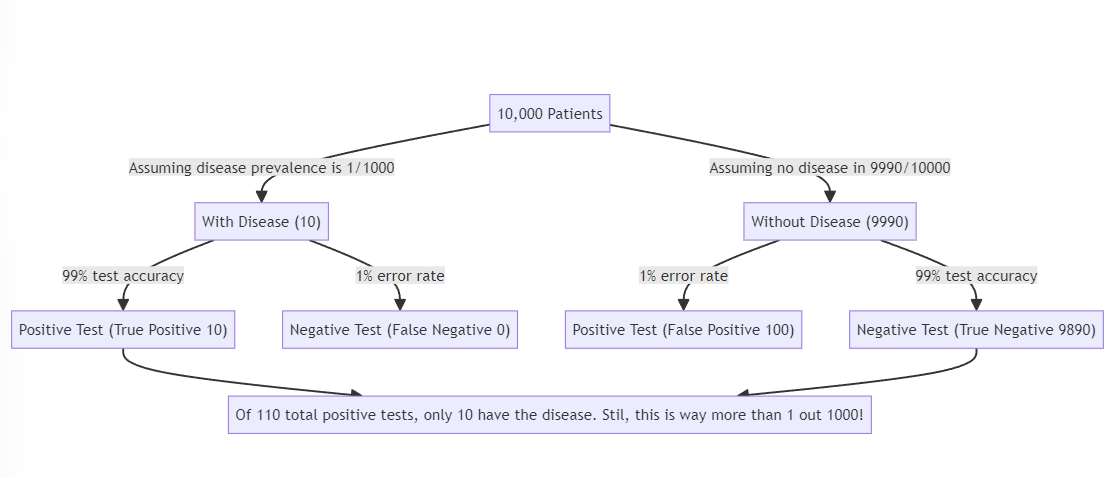
Let’s consider a specific example: a patient takes a test for a rare disease that affects 1 in 1,000 people in the population. The test is 99% accurate, meaning it correctly identifies 99% of people who have the disease (sensitivity) and 99% of people who don’t have the disease (specificity). If the patient tests positive, what is the probability that they actually have the disease?

To answer this question, we can apply Bayes’ Theorem. Let’s define our terms:

H: The hypothesis that the patient has the disease

E: The evidence that the patient tested positive

Pr(H) = 0.001 (the prior probability, or base rate, of having the disease)

Pr(E|H) = 0.99 (the probability of testing positive given that the patient has the disease)

Pr(~H) = 0.999 (the probability of not having the disease)

Pr(E|~H) = 0.01 (the probability of testing positive given that the patient does not have the disease, which is equal to 1 – specificity)

Plugging these values into Bayes’ Theorem:

bayes_theorem(pr_h = 0.001,
pr_e_given_h = 0.99,
pr_e_given_not_h = 0.01)

P(H|E) = (P(E|H) * P(H)) / [P(E|H) * P(H) + P(E|not H) * P(not H)]
= (0.99 * 0.001) / (0.99 * 0.001 + 0.01 * 0.999)
= 0.09

The result might be surprising: even with a highly accurate test and a positive result, there’s only about a 9% chance that the patient actually has the rare disease. This is because the low prior probability of having the disease (the base rate) has a significant impact on the posterior probability.

This example illustrates the importance of considering base rates when interpreting medical test results. Neglecting the base rate can lead to the base rate fallacy, where people overestimate the probability of a condition based on a positive test result without properly accounting for the rarity of the condition in the population.

The base rate fallacy can have serious consequences in medical decision-making. For example, if a doctor overestimates the probability of a patient having a disease based on a positive test result, they might recommend unnecessary treatments or procedures that carry risks and costs. On the other hand, if a doctor underestimates the probability of a disease based on a negative test result, they might fail to provide appropriate care and monitoring.

To avoid the base rate fallacy and make accurate diagnoses, medical professionals (as well as patients and their advocates) must consider both the accuracy of the test and the base rate of the condition in the population. They can use Bayes’ Theorem to update their beliefs about the likelihood of a condition based on the available evidence, just like a detective updating their hypothesis based on clues.

Moreover, medical professionals can use Bayesian reasoning to guide further testing and investigation. If the posterior probability of a condition is still uncertain after an initial test, they can decide whether to order additional tests or gather more information to refine their diagnosis. Each new piece of evidence can be incorporated into the Bayesian framework, allowing for a continual updating of beliefs until a confident diagnosis can be made.

Surprising Applications of Bayes’ Theorem: From Dating to Divinity and Beyond

Bayes’ Theorem is not just a tool for detectives and doctors; it has far-reaching applications in various aspects of life, from the everyday to the extraordinary. Let’s explore some of these surprising applications and see how Bayesian reasoning can help us make better decisions and understand the world around us.

Determining whether to go on a date with someone. When deciding whether to go on a date with someone, you can use Bayes’ Theorem to update your belief about the likelihood of a successful relationship based on the evidence you gather. Your prior probability might be based on your past experiences with relationships or your general beliefs about compatibility. As you learn more about the person through conversations or shared experiences, you can update your probability of a successful relationship. This can help you make a more informed decision about whether to pursue a romantic connection.

Figuring out whether God exists. The question of God’s existence has puzzled philosophers and theologians for centuries. Bayes’ Theorem can provide a framework for updating one’s belief in the existence of God based on evidence and arguments. The prior probability of God’s existence might be based on personal faith or philosophical arguments. Evidence such as the complexity of the universe, the apparent fine-tuning of physical constants, or religious experiences can be incorporated into the Bayesian framework to update the probability of God’s existence. While this approach may not provide a definitive answer, it can help individuals reason about their beliefs in a more structured way.

Determining which scientific theories are true. Science is a process of constantly updating our beliefs based on new evidence. Bayes’ Theorem is a formal way of doing this, allowing scientists to compare the probability of different theories being true based on the available data. The prior probability of a theory might be based on its simplicity, elegance, or consistency with established knowledge. As new experiments are conducted and data is collected, scientists can update the probability of each theory using Bayes’ Theorem. This helps the scientific community converge on the most likely explanations for natural phenomena.

These are just a few examples of the many surprising applications of Bayes’ Theorem. From personal decision-making to the frontiers of science and technology, Bayesian reasoning provides a powerful framework for updating our beliefs in the face of uncertainty. By embracing the principles of Bayesian inference, we can make more informed choices, uncover hidden truths, and push the boundaries of what is possible.

Sample Problems

Please anwser these questions using the bayes_theorem function.

You are a detective investigating a burglary. Based on your initial assessment of the crime scene, you believe there is a 60% chance that the burglar entered through the front door. However, upon further investigation, you discover that the lock on the back door was picked, and there are muddy footprints leading from the back door to the area where the valuables were stolen. Given this new evidence, how would you update your belief about the burglar’s entry point using Bayes’ Theorem?

# You’ll need to replace the ? with the right numbers
bayes_theorem(pr_h = ?,
pr_e_given_h = ?,
pr_e_given_not_h = ?)

A certain disease affects 1 in 10,000 people. A test for this disease has a 95% accuracy rate, meaning it correctly identifies 95% of people who have the disease and 95% of people who don’t have the disease. If a person tests positive for the disease, what is the probability that they actually have the disease? Use Bayes’ Theorem to calculate the updated probability.

# You’ll need to replace the ? with the right numbers
bayes_theorem(pr_h = ?,
pr_e_given_h = ?,
pr_e_given_not_h = ?)

You are considering whether to go on a date with someone you met online. Based on their profile and your prior experiences with online dating, you initially believe there is a 30% chance that you will have a good connection in person. After exchanging a few messages, you discover that you have several shared interests and values. Given this new information, how would you update your belief about the likelihood of a successful date using Bayes’ Theorem?

# You’ll need to replace the ? with the right numbers
bayes_theorem(pr_h = ?,
pr_e_given_h = ?,
pr_e_given_not_h = ?)

Minds that Mattered: Florence Nightingale

Florence Nightingale (1820-1910) was a British nurse, statistician, and social reformer who revolutionized healthcare practices in the 19th century. Born in Florence, Italy, to a wealthy British family, Nightingale was well-educated and had a strong interest in mathematics and statistics from a young age. Despite her family’s objections, she pursued a career in nursing, which was considered an unsuitable profession for a woman of her social standing at the time.

Nightingale’s most notable contribution came during the Crimean War (1853-1856), where she served as a nurse in military hospitals. She was appalled by the unsanitary conditions, lack of medical supplies, and high mortality rates among the wounded soldiers. Nightingale worked tirelessly to improve the hospitals, implementing strict hygiene protocols, ensuring proper ventilation, and providing adequate food and medical care. Her dedication and compassion earned her the nickname “The Lady with the Lamp,” as she would often make night rounds to check on her patients.

After returning from the Crimean War, Nightingale continued her mission to reform healthcare. She used her statistical knowledge to analyze mortality data and demonstrate the link between sanitary conditions and patient outcomes. Nightingale’s findings led to significant improvements in hospital design, sanitation practices, and patient care.

Key Ideas

Evidence-Based Medicine. Florence Nightingale strongly believed in the importance of collecting and analyzing data to inform healthcare practices. She meticulously recorded and analyzed patient outcomes, mortality rates, and hospital conditions. Nightingale’s evidence-based approach laid the foundation for modern medical research and emphasized the importance of data-driven decision making in healthcare.

Data Visualization. Nightingale was a pioneer in data visualization. She created the polar area diagram, also known as the Nightingale Rose Diagram, to visually represent the causes of mortality in the Crimean War hospitals. The diagram used segmented circles to show the proportion of deaths due to preventable causes, such as infectious diseases, compared to other causes. This innovative visual representation made complex statistical data accessible to a wider audience and helped convince authorities to implement hospital reforms.

Nursing Education. Nightingale recognized the need for formal training and education for nurses. In 1860, she established the Nightingale Training School for Nurses at St. Thomas’ Hospital in London. The school provided a rigorous curriculum that combined theoretical knowledge with practical training. Nightingale’s model of nursing education emphasized the importance of hygiene, patient observation, and evidence-based practices. The Nightingale Training School set the standard for modern nursing education and helped elevate nursing to a respected profession.

Influence

Florence Nightingale’s influence extends across multiple fields, including nursing, public health, and data science.

In nursing, Nightingale’s reforms transformed the profession from a low-skilled, often disreputable occupation to a highly respected and essential role in healthcare. Her emphasis on hygiene, patient care, and evidence-based practices laid the foundation for modern nursing standards. Nightingale’s legacy continues to inspire nurses worldwide, and International Nurses Day is celebrated on her birthday, May 12th, in her honor.

In public health, Nightingale’s work highlighted the importance of sanitation and hygiene in preventing the spread of infectious diseases. Her reforms in hospital design and sanitation practices led to significant reductions in mortality rates and improved patient outcomes. Nightingale’s advocacy for public health measures, such as improved sanitation and access to clean water, had a lasting impact on population health.

In data science, Nightingale’s innovative use of statistics and data visualization to identify healthcare problems and drive reforms established her as a pioneer in the field. Her Nightingale Rose Diagram showcased the power of visual representations in communicating complex data and influencing policy decisions. Nightingale’s work laid the groundwork for the use of statistical analysis in healthcare and inspired future generations of data scientists.

Review Questions

What were the primary challenges Florence Nightingale faced during the Crimean War, and how did she address them?

Explain the significance of evidence-based medicine in Nightingale’s approach to healthcare reform.

How did Nightingale’s data visualization techniques, such as the Nightingale Rose Diagram, contribute to her advocacy for hospital reforms?

Discuss the impact of the Nightingale Training School for Nurses on the nursing profession and nursing education.

In what ways did Florence Nightingale’s work influence the fields of public health and data science?

Glossary

Here is a glossary of some helpful terms.

Term	Definition
Probability	A numerical measure of the likelihood that an event will occur, expressed as a value between 0 and 1, where 0 indicates impossibility and 1 indicates certainty.
Complement Rule	States that the probability of an event not occurring is equal to 1 minus the probability of the event occurring. Mathematically, for an event A, P(A’) = 1 – P(A).
Simple Addition Rule (for mutually exclusive events)	States that the probability of either of two mutually exclusive events occurring is equal to the sum of their individual probabilities. Mathematically, for mutually exclusive events A and B, P(A or B) = P(A) + P(B).
General Addition Rule	States that the probability of at least one of two events occurring is equal to the sum of their individual probabilities minus the probability of both events occurring simultaneously. Mathematically, for events A and B, P(A or B) = P(A) + P(B) – P(A and B).
Simple Multiplication Rule (for independent events)	States that the probability of two independent events both occurring is equal to the product of their individual probabilities. Mathematically, for independent events A and B, P(A and B) = P(A) × P(B).
General Multiplication Rule	States that the probability of two events both occurring is equal to the probability of one event occurring multiplied by the conditional probability of the second event occurring given that the first event has occurred. Mathematically, for events A and B, P(A and B) = P(A) × P(B
Conditional Probability	The probability of an event occurring given that another event has already occurred. Mathematically, for events A and B, the conditional probability of A given B is denoted as P(A
Rule of Total Probability	A formula that expresses the total probability of an event as the sum of the products of the conditional probabilities of the event given each possible outcome of another event and the probabilities of those outcomes. Mathematically, if B1, B2, …, Bn are mutually exclusive and exhaustive events, then for any event A, P(A) = P(A
Frequency-type probability	An interpretation of probability based on the relative frequency of an event occurring in a large number of trials or observations.
Belief-type probability	An interpretation of probability based on an individual’s subjective belief or confidence in the likelihood of an event occurring, often informed by prior knowledge or experience.
Bayes Theorem	A formula that describes the relationship between conditional probabilities and enables the updating of probabilities based on new evidence or information. Mathematically, for events A and B, Bayes Theorem states that P(A
Prior Probability – Pr(H)	The initial probability of a hypothesis (H) being true before considering any evidence or data.
Posterior Probability – Pr(H|E)	The updated probability of a hypothesis (H) being true after considering the evidence (E) or data.
Likelihood – Pr(E|H)	The probability of observing the evidence (E) given that the hypothesis (H) is true.
Pr(E| not H)	The probability of observing the evidence (E) given that the hypothesis (H) is not true.

References

Carnap, Rudolf. 1945. “The Two Concepts of Probability: The Problem of Probability.” Philosophy and Phenomenological Research 5 (4): 513-532. https://www.jstor.org/stable/2102817.

Crane, Harry. 2016. “Probability.” Internet Encyclopedia of Philosophy. https://iep.utm.edu/prob-ind/.

Fitelson, Branden. 2006. “Inductive Logic.” Stanford Encyclopedia of Philosophy. https://plato.stanford.edu/entries/logic-inductive/.

Hájek, Alan. 2019. “Interpretations of Probability.” Stanford Encyclopedia of Philosophy. https://plato.stanford.edu/entries/probability-interpret/.

Huber, Franz. 2016. “Formal Representations of Belief.” Stanford Encyclopedia of Philosophy. https://plato.stanford.edu/entries/formal-belief/.

Joyce, James. 2003. “Bayes’ Theorem.” Stanford Encyclopedia of Philosophy. https://plato.stanford.edu/entries/bayes-theorem/.

Leighton, Jonathan P. 2017. “Logic and Probability.” In The Oxford Handbook of Philosophical Methodology, edited by Herman Cappelen, Tamar Szabó Gendler, and John Hawthorne. Oxford: Oxford University Press.

Talbott, William. 2016. “Bayesian Epistemology.” Stanford Encyclopedia of Philosophy. https://plato.stanford.edu/entries/epistemology-bayesian/.

The Probability and Statistics Cookbook. n.d. Matthias Vallentin. http://statistics.zone/.

Vickers, John. 2016. “The Problem of Induction.” Stanford Encyclopedia of Philosophy. https://plato.stanford.edu/entries/induction-problem/.

Vineberg, Susan. 2011. “Dutch Book Arguments.” Stanford Encyclopedia of Philosophy. https://plato.stanford.edu/entries/dutch-book/.

Weisberg, Jonathan. 2011. “Varieties of Bayesianism.” In Handbook of the History of Logic. Vol. 10: Inductive Logic, edited by Dov M. Gabbay, Stephan Hartmann, and John Woods, 477-551. Amsterdam: Elsevier.

Probability and Statistics. n.d. Khan Academy. https://www.khanacademy.org/math/statistics-probability.